Theory
This section develops the theoretical foundations of panel data econometrics, focusing on the fixed effects estimator and its properties.
The Panel Data Model
Setup
We observe \(N\) units (countries) over \(T\) time periods (quarters). The data generating process (DGP) is:
\[
y_{it} = \mathbf{x}_{it}'\boldsymbol{\beta} + \alpha_i + \varepsilon_{it}, \quad i = 1, \ldots, N, \quad t = 1, \ldots, T
\]
where:
- \(y_{it}\): outcome (e.g., policy rate for country \(i\) at time \(t\))
- \(\mathbf{x}_{it}\): \(K \times 1\) vector of observable regressors (e.g., bank holdings, inflation)
- \(\boldsymbol{\beta}\): \(K \times 1\) parameter vector of interest
- \(\alpha_i\): unobserved time-invariant individual effect (institutions, geography, political culture)
- \(\varepsilon_{it}\): idiosyncratic error
The key question: what happens to \(\hat{\boldsymbol{\beta}}\) when we ignore \(\alpha_i\)?
Pooled OLS: The Naive Approach
If we ignore the panel structure and estimate by OLS:
\[
y_{it} = \mathbf{x}_{it}'\boldsymbol{\beta} + u_{it}, \quad \text{where } u_{it} = \alpha_i + \varepsilon_{it}
\]
The OLS estimator is:
\[
\hat{\boldsymbol{\beta}}_{\text{OLS}} = \left(\sum_{i=1}^{N}\sum_{t=1}^{T} \mathbf{x}_{it}\mathbf{x}_{it}'\right)^{-1} \left(\sum_{i=1}^{N}\sum_{t=1}^{T} \mathbf{x}_{it} y_{it}\right)
\]
Consistency requires \(\text{plim} \left(\frac{1}{NT}\sum_{i,t} \mathbf{x}_{it} u_{it}\right) = \mathbf{0}\).
Expanding: \[
\frac{1}{NT}\sum_{i,t} \mathbf{x}_{it} u_{it} = \frac{1}{NT}\sum_{i,t} \mathbf{x}_{it} \alpha_i + \frac{1}{NT}\sum_{i,t} \mathbf{x}_{it} \varepsilon_{it}
\]
The second term vanishes under standard exogeneity (\(E[\varepsilon_{it}|\mathbf{x}_{it}] = 0\)). But the first term:
\[
\frac{1}{NT}\sum_{i,t} \mathbf{x}_{it} \alpha_i \xrightarrow{p} E[\mathbf{x}_{it} \alpha_i] = \text{Cov}(\mathbf{x}_{it}, \alpha_i) + E[\mathbf{x}_{it}]E[\alpha_i]
\]
If \(\text{Cov}(\mathbf{x}_{it}, \alpha_i) \neq 0\), pooled OLS is inconsistent.
In macroeconomic panels, countries with high bank holdings of sovereign debt (\(\mathbf{x}\)) likely have different institutional quality (\(\alpha\)) than countries with low holdings. A banking system may hold lots of government bonds because of institutional features (regulatory requirements, underdeveloped capital markets) that also independently affect monetary policy. Pooled OLS conflates the causal effect of bank holdings with these institutional differences.
The Fixed Effects Estimator
What FE Uses and What It Discards
FE uses only within-unit variation: deviations of \(x_{it}\) from its country mean \(\bar{x}_i\).
- If a country always has bank holdings of 30%, it contributes zero identifying variation to \(\hat{\beta}_{\text{FE}}\)
- The identifying variation comes from changes in bank holdings within a country over time
- A country that goes from 20% to 35% holdings contributes a lot; a country stuck at 25% contributes little
FE discards between-unit variation: differences in average \(\bar{x}_i\) across countries.
This is both the strength (eliminates \(\alpha_i\) bias) and the weakness (throws away cross-sectional information, reduces efficiency).
Consistency
\(\hat{\boldsymbol{\beta}}_{\text{FE}}\) is consistent under:
Assumption (Strict Exogeneity): \[
E[\varepsilon_{it} | \mathbf{x}_{i1}, \ldots, \mathbf{x}_{iT}, \alpha_i] = 0 \quad \forall \, t
\]
This means:
- Current errors are uncorrelated with past, present, AND future regressors
- This rules out feedback effects: if past \(y\) affects current \(x\), strict exogeneity fails
- This also rules out lagged dependent variables as regressors (Nickell bias)
The Frisch-Waugh-Lovell Theorem
The FE estimator is numerically identical to OLS with \(N\) country dummies.
Theorem (Frisch-Waugh-Lovell): In the regression \(y = X_1\beta_1 + X_2\beta_2 + \varepsilon\), the OLS estimate of \(\beta_1\) is identical to the OLS estimate from regressing \(M_2 y\) on \(M_2 X_1\), where \(M_2 = I - X_2(X_2'X_2)^{-1}X_2'\) is the annihilator matrix for \(X_2\).
Application to FE: Let \(X_1 = \mathbf{X}\) (regressors of interest) and \(X_2 = D\) (matrix of country dummies). Then:
- \(M_D \mathbf{x}_{it} = \mathbf{x}_{it} - \bar{\mathbf{x}}_i = \ddot{\mathbf{x}}_{it}\) (the within transformation!)
- \(M_D y_{it} = y_{it} - \bar{y}_i = \ddot{y}_{it}\)
So FE = OLS with dummies = OLS on demeaned data. These are algebraically identical.
Practical implication: fixest::feols() uses the within transformation (fast), while lm() with dummy variables estimates all \(N\) dummy coefficients (slow, memory-intensive). Same \(\hat{\beta}\), different computational cost.
Two-Way Fixed Effects
The Model
\[
y_{it} = \mathbf{x}_{it}'\boldsymbol{\beta} + \alpha_i + \lambda_t + \varepsilon_{it}
\]
Now \(\lambda_t\) absorbs time-varying shocks common to all units:
- \(\alpha_i\): Country A is different from Country B in time-invariant ways
- \(\lambda_t\): 2022Q2 was different from 2019Q2 for all countries (global inflation surge, Fed tightening)
Double Demeaning
The two-way within transformation removes both \(\alpha_i\) and \(\lambda_t\):
\[
\tilde{y}_{it} = y_{it} - \bar{y}_{i\cdot} - \bar{y}_{\cdot t} + \bar{y}_{\cdot\cdot}
\]
What’s left: \(\tilde{y}_{it}\) is the part of \(y_{it}\) that can’t be explained by country-level or time-level averages. It’s the country-specific deviation from the global trend.
What Each Fixed Effect Absorbs
| Country FE (\(\alpha_i\)) |
All time-invariant country differences |
Regulatory frameworks, reserve currency status |
| Time FE (\(\lambda_t\)) |
All country-invariant time shocks |
Global inflation surge, commodity price spikes |
| Neither |
Country-specific, time-varying variation |
Country A’s holdings rose more in 2020 than average |
Interactions in Panel Models
The Interaction Term
Consider a specification with an interaction:
\[
y_{it} = \gamma_1 x_{it} + \gamma_2 z_{it} + \gamma_3 (x_{it} \times z_{it}) + \alpha_i + \lambda_t + \varepsilon_{it}
\]
What does \(\gamma_3\) mean?
The marginal effect of \(x\) on \(y\) is:
\[
\frac{\partial y_{it}}{\partial x_{it}} = \gamma_1 + \gamma_3 \cdot z_{it}
\]
This is not constant—it depends on the level of \(z_{it}\).
If \(\gamma_1 > 0\) and \(\gamma_3 < 0\), there exists a “crossing point” \(z^* = -\gamma_1/\gamma_3\) where the marginal effect of \(x\) switches sign. Below \(z^*\), \(x\) has a positive effect; above \(z^*\), negative.
Clustering Standard Errors
Standard OLS assumes \(\varepsilon_{it}\) is i.i.d. This fails in panels because:
- Serial correlation within country: A country’s error in 2022Q1 is correlated with its error in 2022Q2
- Cross-sectional dependence: Country A’s error in 2022Q1 may correlate with Country B’s (global shocks)
Clustering by country handles (1): it allows arbitrary within-country correlation over time.
Important: Cluster-robust inference requires \(N \to \infty\). With only 30 countries, cluster SEs may be unreliable. Rule of thumb: need \(N \geq 50\) for good coverage. With small \(N\), consider wild cluster bootstrap.
Monte Carlo Simulations
This section uses Monte Carlo simulations to demonstrate the properties of panel estimators.
Demonstrating OVB: Pooled OLS vs. FE
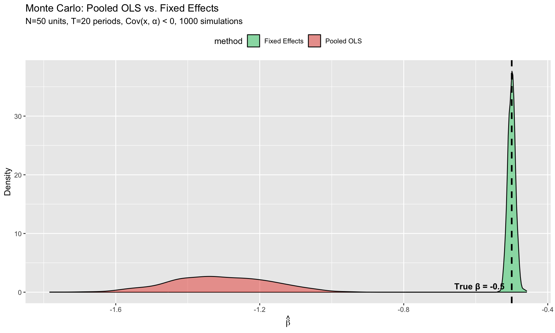
We simulate a panel where \(\text{Cov}(x_{it}, \alpha_i) \neq 0\) and show that pooled OLS is biased while FE is consistent.
set.seed(42)

# Parameters
N <- 50       # countries
T_per <- 20   # quarters
beta_true <- -0.5  # true effect: negative
gamma_alpha <- 3   # how much alpha matters for y

# Simulation
n_sims <- 1000
beta_ols <- numeric(n_sims)
beta_fe  <- numeric(n_sims)

for (s in 1:n_sims) {
  # Generate unobserved heterogeneity
  alpha <- rnorm(N, mean = 5, sd = 2)  # country effect

  # Generate x correlated with alpha
  # Countries with higher alpha have LOWER x (negative correlation)
  x <- matrix(NA, N, T_per)
  for (i in 1:N) {
    x[i, ] <- -0.8 * alpha[i] + rnorm(T_per, mean = 20, sd = 3)
  }

  # Generate y
  y <- matrix(NA, N, T_per)
  eps <- matrix(rnorm(N * T_per, sd = 1), N, T_per)
  for (i in 1:N) {
    y[i, ] <- beta_true * x[i, ] + gamma_alpha * alpha[i] + eps[i, ]
  }

  # Reshape to panel
  id <- rep(1:N, each = T_per)
  tt <- rep(1:T_per, times = N)
  yy <- as.vector(t(y))
  xx <- as.vector(t(x))

  # Pooled OLS
  beta_ols[s] <- coef(lm(yy ~ xx))[2]

  # Fixed Effects
  df <- data.frame(y = yy, x = xx, id = factor(id))
  beta_fe[s] <- coef(fixest::feols(y ~ x | id, data = df))["x"]
}

# Results
cat("=== Monte Carlo Results (1000 simulations) ===\n")
=== Monte Carlo Results (1000 simulations) ===
cat(sprintf("True beta: %.3f\n", beta_true))
cat(sprintf("Pooled OLS mean: %.3f (bias = %.3f)\n", mean(beta_ols), mean(beta_ols) - beta_true))
Pooled OLS mean: -1.310 (bias = -0.810)
cat(sprintf("FE mean: %.3f (bias = %.3f)\n", mean(beta_fe), mean(beta_fe) - beta_true))
FE mean: -0.500 (bias = -0.000)
df_mc <- data.frame(
  estimate = c(beta_ols, beta_fe),
  method = rep(c("Pooled OLS", "Fixed Effects"), each = n_sims)
)

ggplot(df_mc, aes(x = estimate, fill = method)) +
  geom_density(alpha = 0.5) +
  geom_vline(xintercept = beta_true, linetype = "dashed", linewidth = 1) +
  annotate("text", x = beta_true - 0.02, y = 0, label = paste("True β =", beta_true),
           hjust = 1, vjust = -0.5, fontface = "bold") +
  labs(
    title = "Monte Carlo: Pooled OLS vs. Fixed Effects",
    subtitle = "N=50 units, T=20 periods, Cov(x, α) < 0, 1000 simulations",
    x = expression(hat(beta)),
    y = "Density"
  ) +
  scale_fill_manual(values = c("Pooled OLS" = "#e74c3c", "Fixed Effects" = "#2ecc71")) +
  theme(legend.position = "top")
What you should see: The OLS distribution is centered well above the true value (biased positive). The FE distribution is centered on the truth.
Demonstrating Time FE Importance
set.seed(123)

N <- 40
T_per <- 20
beta_true <- -0.3

n_sims <- 500
beta_country_fe <- numeric(n_sims)
beta_twoway_fe  <- numeric(n_sims)

for (s in 1:n_sims) {
  alpha <- rnorm(N, sd = 3)         # country effects
  lambda <- rnorm(T_per, sd = 2)    # time effects

  # x correlated with both alpha AND lambda
  x <- matrix(NA, N, T_per)
  for (i in 1:N) {
    for (t in 1:T_per) {
      x[i, t] <- -0.5 * alpha[i] + 0.4 * lambda[t] + rnorm(1, mean = 20, sd = 2)
    }
  }

  y <- matrix(NA, N, T_per)
  for (i in 1:N) {
    for (t in 1:T_per) {
      y[i, t] <- beta_true * x[i, t] + alpha[i] + lambda[t] + rnorm(1, sd = 1)
    }
  }

  id <- rep(1:N, each = T_per)
  tt <- rep(1:T_per, times = N)
  df <- data.frame(y = as.vector(t(y)), x = as.vector(t(x)),
                   id = factor(id), time = factor(tt))

  beta_country_fe[s] <- coef(feols(y ~ x | id, data = df))["x"]
  beta_twoway_fe[s]  <- coef(feols(y ~ x | id + time, data = df))["x"]
}

cat("=== Time FE Matters When x Correlates with Time Shocks ===\n")
=== Time FE Matters When x Correlates with Time Shocks ===
cat(sprintf("True beta: %.3f\n", beta_true))
cat(sprintf("Country FE only:     %.3f  (bias = %.3f)\n",
            mean(beta_country_fe), mean(beta_country_fe) - beta_true))
Country FE only: 0.045 (bias = 0.345)
cat(sprintf("Two-way FE:          %.3f  (bias = %.3f)\n",
            mean(beta_twoway_fe), mean(beta_twoway_fe) - beta_true))
Two-way FE: -0.300 (bias = -0.000)
Key lesson: Country FE alone is not enough if the regressors correlate with common time shocks.
Cluster SE Coverage
set.seed(99)

N <- 30     # small number of clusters
T_per <- 12
beta_true <- -0.5

n_sims <- 1000
cover_iid <- 0
cover_cluster <- 0

for (s in 1:n_sims) {
  alpha <- rnorm(N, sd = 3)

  # Generate x and y with serially correlated errors
  x <- matrix(NA, N, T_per)
  y <- matrix(NA, N, T_per)
  for (i in 1:N) {
    x[i, ] <- -0.5 * alpha[i] + rnorm(T_per, 20, 3)
    eps <- arima.sim(list(ar = 0.6), n = T_per, sd = 1)  # AR(1) errors
    y[i, ] <- beta_true * x[i, ] + alpha[i] + eps
  }

  df <- data.frame(y = as.vector(t(y)), x = as.vector(t(x)),
                   id = factor(rep(1:N, each = T_per)))

  fit <- feols(y ~ x | id, data = df)

  # IID standard errors
  ci_iid <- confint(fit, se = "iid")
  cover_iid <- cover_iid + (ci_iid[1] <= beta_true & beta_true <= ci_iid[2])

  # Cluster standard errors
  ci_cluster <- confint(fit, cluster = ~id)
  cover_cluster <- cover_cluster + (ci_cluster[1] <= beta_true & beta_true <= ci_cluster[2])
}

cat("=== 95% CI Coverage (AR(1) errors within clusters) ===\n")
=== 95% CI Coverage (AR(1) errors within clusters) ===
cat(sprintf("IID SEs: %.1f%% (should be 95%%)\n", 100 * cover_iid / n_sims))
IID SEs: 95.7% (should be 95%)
cat(sprintf("Cluster SEs: %.1f%% (should be 95%%)\n", 100 * cover_cluster / n_sims))
Cluster SEs: 95.4% (should be 95%)
What you should see: IID standard errors have coverage well below 95% (too many false positives). Cluster SEs restore correct coverage.
Application
This section applies the methods to macroeconomic panel data.
Data Preparation
# Prepare the analysis sample
analysis <- master %>%
  mutate(quarter = as.integer(gsub(".*Q", "", year_quarter))) %>%
  group_by(country) %>%
  arrange(year, quarter) %>%
  mutate(
    # Lagged variables
    L1_bank_holdings_pct = lag(bank_holdings_pct),
    L1_cb_holdings_pct = lag(cb_holdings_pct)
  ) %>%
  ungroup() %>%
  filter(!is.na(policy_rate), !is.na(bank_holdings_pct))

# Post-2022 subsample
tightening <- analysis %>%
  filter(year >= 2022) %>%
  filter(!is.na(L1_bank_holdings_pct))

cat("Full sample:", nrow(analysis), "obs,", n_distinct(analysis$country), "countries\n")
Full sample: 3406 obs, 41 countries
cat("Post-2022 sample:", nrow(tightening), "obs,", n_distinct(tightening$country), "countries\n")
Post-2022 sample: 480 obs, 40 countries
Building Up: OLS → FE → TWFE
# Check if we have the necessary variables
if ("inflation_yoy" %in% names(tightening) || "sovereign_debt_gdp" %in% names(tightening)) {

  # Step 1: Pooled OLS
  m1 <- feols(policy_rate ~ L1_bank_holdings_pct + sovereign_debt_gdp,
              data = tightening)

  # Step 2: Country FE only
  m2 <- feols(policy_rate ~ L1_bank_holdings_pct | country,
              data = tightening)

  # Step 3: Two-way FE
  m3 <- feols(policy_rate ~ L1_bank_holdings_pct | country + year_quarter,
              data = tightening)

  # Step 4: Add CB holdings
  m4 <- feols(policy_rate ~ L1_bank_holdings_pct + L1_cb_holdings_pct
              | country + year_quarter,
              data = tightening)

  # Step 5: Interaction
  m5 <- feols(policy_rate ~ L1_bank_holdings_pct * L1_cb_holdings_pct
              | country + year_quarter,
              data = tightening)

  # Display with appropriate SEs
  # Note: In practice, FE models should use clustered SEs
  etable(m1, m2, m3, m4, m5,
         headers = c("Pooled", "Country FE", "TWFE", "+CB", "Interaction"),
         vcov = list("iid", ~country, ~country, ~country, ~country),
         fitstat = ~ n + r2 + wr2)
} else {
  cat("Note: Full specification requires inflation and debt variables.\n")
  cat("Running simplified demonstration with available variables.\n")

  m1 <- feols(policy_rate ~ L1_bank_holdings_pct, data = tightening)
  m2 <- feols(policy_rate ~ L1_bank_holdings_pct | country, data = tightening)
  m3 <- feols(policy_rate ~ L1_bank_holdings_pct | country + year_quarter, data = tightening)

  etable(m1, m2, m3,
         headers = c("Pooled", "Country FE", "TWFE"),
         vcov = list("iid", ~country, ~country),
         fitstat = ~ n + r2 + wr2)
}
                                                          m1              m2
                                                      Pooled      Country FE
Dependent Var.:                                  policy_rate     policy_rate

Constant                                    7.886*** (1.510)
L1_bank_holdings_pct                        0.0687. (0.0369) 0.3734 (0.6231)
sovereign_debt_gdp                        -0.0402** (0.0146)
L1_cb_holdings_pct
L1_bank_holdings_pct x L1_cb_holdings_pct
Fixed-Effects:                            ------------------ ---------------
country                                                   No             Yes
year_quarter                                              No              No
________________________________________  __________________ _______________
S.E. type                                                IID     by: country
Observations                                             480             480
R2                                                   0.02667         0.81188
Within R2                                                 --         0.00812

                                                       m3              m4
                                                     TWFE             +CB
Dependent Var.:                               policy_rate     policy_rate

Constant
L1_bank_holdings_pct                      0.5777 (0.6425) 0.6562 (0.6863)
sovereign_debt_gdp
L1_cb_holdings_pct                                        0.5837 (0.6104)
L1_bank_holdings_pct x L1_cb_holdings_pct
Fixed-Effects:                            --------------- ---------------
country                                               Yes             Yes
year_quarter                                          Yes             Yes
________________________________________  _______________ _______________
S.E. type                                     by: country     by: country
Observations                                          480             480
R2                                                0.83693         0.84322
Within R2                                         0.02141         0.05916

                                                       m5
                                              Interaction
Dependent Var.:                               policy_rate

Constant
L1_bank_holdings_pct                      0.4222 (0.3321)
sovereign_debt_gdp
L1_cb_holdings_pct                        0.2438 (0.4371)
L1_bank_holdings_pct x L1_cb_holdings_pct 0.0201 (0.0386)
Fixed-Effects:                            ---------------
country                                               Yes
year_quarter                                          Yes
________________________________________  _______________
S.E. type                                     by: country
Observations                                          480
R2                                                0.84451
Within R2                                         0.06693
---
Signif. codes: 0 '***' 0.001 '**' 0.01 '*' 0.05 '.' 0.1 ' ' 1
Within-Country Variation
within_var <- tightening %>%
  group_by(country) %>%
  summarise(
    mean_holdings = mean(L1_bank_holdings_pct, na.rm = TRUE),
    sd_within = sd(L1_bank_holdings_pct, na.rm = TRUE),
    range_within = max(L1_bank_holdings_pct, na.rm = TRUE) -
                   min(L1_bank_holdings_pct, na.rm = TRUE),
    n_obs = n()
  ) %>%
  arrange(desc(sd_within))

cat("=== Within-Country Variation ===\n")
=== Within-Country Variation ===
print(head(within_var, 5))
# A tibble: 5 × 5
  country   mean_holdings sd_within range_within n_obs
  <chr>             <dbl>     <dbl>        <dbl> <int>
1 Argentina         20.7       2.94         8.95    12
2 Turkey            56.8       2.65         9.22    12
3 Denmark            6.33      2.37         7.61    12
4 Sweden            35.7       2.26         9.05    12
5 Hungary           25.3       2.22         6.39    12
# Variance decomposition
between_var <- var(within_var$mean_holdings, na.rm = TRUE)
avg_within_var <- mean(within_var$sd_within^2, na.rm = TRUE)
total_var <- var(tightening$L1_bank_holdings_pct, na.rm = TRUE)

cat(sprintf("\n=== Variance Decomposition ===\n"))
=== Variance Decomposition ===
cat(sprintf("Between variance: %.0f%%\n", 100 * between_var / total_var))
cat(sprintf("Within variance: %.0f%%\n", 100 * avg_within_var / total_var))
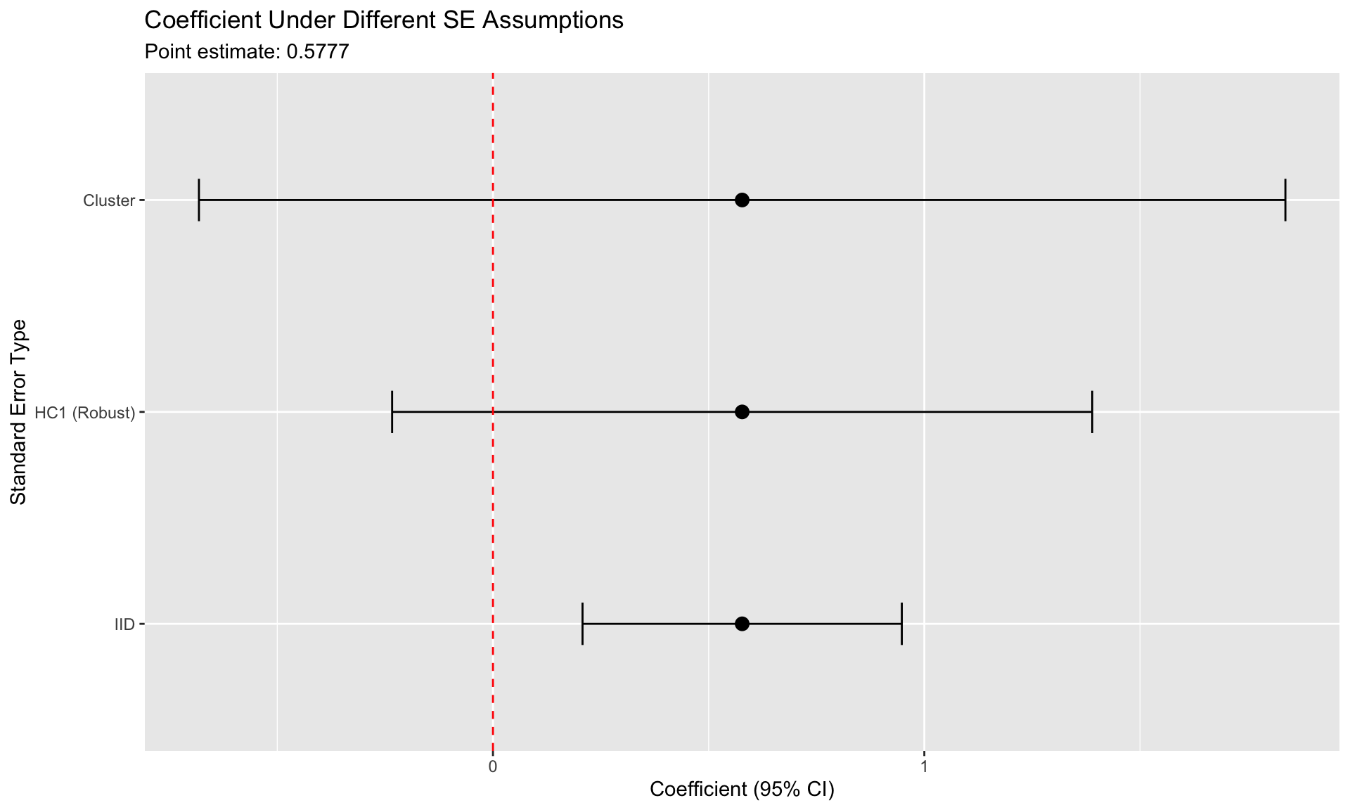
Standard Error Comparison
m_main <- feols(policy_rate ~ L1_bank_holdings_pct | country + year_quarter,
                data = tightening)

coef_name <- "L1_bank_holdings_pct"
coef_val <- coef(m_main)[coef_name]

se_types <- c("IID", "HC1 (Robust)", "Cluster")
se_vals <- c(
  sqrt(vcov(m_main, se = "iid")[coef_name, coef_name]),
  sqrt(vcov(m_main, se = "hetero")[coef_name, coef_name]),
  sqrt(vcov(m_main, cluster = ~country)[coef_name, coef_name])
)

se_df <- data.frame(
  type = factor(se_types, levels = se_types),
  se = se_vals,
  lower = coef_val - 1.96 * se_vals,
  upper = coef_val + 1.96 * se_vals
)

ggplot(se_df, aes(x = type, y = coef_val)) +
  geom_point(size = 3) +
  geom_errorbar(aes(ymin = lower, ymax = upper), width = 0.2) +
  geom_hline(yintercept = 0, linetype = "dashed", color = "red") +
  labs(
    title = "Coefficient Under Different SE Assumptions",
    subtitle = paste("Point estimate:", round(coef_val, 4)),
    x = "Standard Error Type",
    y = "Coefficient (95% CI)"
  ) +
  coord_flip()
Frequently Asked Questions
Common conceptual questions when working with panel fixed effects.
Why not random effects?
The Hausman test typically rejects RE in favor of FE in macro panels. More importantly, RE assumes \(\text{Cov}(\mathbf{x}_{it}, \alpha_i) = 0\), which is often implausible: units with high values of the regressor may differ systematically from units with low values in ways that affect the outcome. FE is the safer choice when this correlation is likely.
What if within R² is low?
Within \(R^2\) in two-way FE models is supposed to be low. The overall \(R^2\) is often 70%+, with most explained by fixed effects. Within \(R^2\) measures how much of the remaining variation our regressors explain. In macro panels, a within \(R^2\) of 3-8% is normal. Statistical significance of coefficients is what matters for testing hypotheses.
What about endogeneity?
Fixed effects address endogeneity from time-invariant confounders. For time-varying endogeneity, consider:
- Instrumental variables (Module 2)
- Placebo tests in pre-treatment periods
- Timing variation within treated groups
- Lagged regressors (with caution about Nickell bias)
Summary
Key takeaways from this module:
Pooled OLS is biased when unobserved heterogeneity correlates with regressors
FE uses only within-unit variation — conservative but credible
Two-way FE absorbs global shocks — your coefficient captures country-specific deviations from global trends
Interactions reveal mechanisms — the effect of one variable may depend on another
Cluster your standard errors — IID SEs are too small due to within-country correlation
Low within R² is expected — the question is whether the mechanism is detectable, not whether it explains all variation
Next: Module 2: Identification in Macroeconomics