Bayesian Foundations

From Priors to Posteriors in Macroeconometrics

The Bayesian Paradigm

Bayesian inference provides a coherent framework for combining prior knowledge with data to quantify uncertainty about parameters. In macroeconometrics, where samples are small and prior information is often available, Bayesian methods have become essential.

Bayes’ Theorem

The foundation of Bayesian inference:

\[ \underbrace{p(\theta | Y)}_{\text{Posterior}} = \frac{\overbrace{p(Y | \theta)}^{\text{Likelihood}} \times \overbrace{p(\theta)}^{\text{Prior}}}{\underbrace{p(Y)}_{\text{Marginal Likelihood}}} \]

Or, since \(p(Y)\) is a constant given the data:

\[ p(\theta | Y) \propto p(Y | \theta) \times p(\theta) \]

In words: What we believe after seeing the data (posterior) is proportional to what the data tells us (likelihood) times what we believed before (prior).

Code
# Demonstrate Bayesian updating
# Example: estimating a mean with known variance

# True parameter
theta_true <- 2.5

# Prior: N(0, 1) - vague prior centered at 0
prior_mean <- 0
prior_var <- 1

# Data: 5 observations with known variance
n <- 5
sigma2 <- 1  # known variance
y <- rnorm(n, theta_true, sqrt(sigma2))
y_bar <- mean(y)

# Posterior (conjugate update)
# For normal-normal: posterior_mean = weighted average
# posterior_var = 1/(1/prior_var + n/sigma2)
post_var <- 1 / (1/prior_var + n/sigma2)
post_mean <- post_var * (prior_mean/prior_var + n*y_bar/sigma2)

# Plot
theta_grid <- seq(-2, 5, length.out = 500)

plot_data <- data.frame(
  theta = rep(theta_grid, 3),
  density = c(
    dnorm(theta_grid, prior_mean, sqrt(prior_var)),
    dnorm(theta_grid, y_bar, sqrt(sigma2/n)) * 2,  # scaled likelihood
    dnorm(theta_grid, post_mean, sqrt(post_var))
  ),
  type = rep(c("Prior", "Likelihood (scaled)", "Posterior"), each = length(theta_grid))
)

ggplot(plot_data, aes(x = theta, y = density, color = type, linetype = type)) +
  geom_line(size = 1.2) +
  geom_vline(xintercept = theta_true, linetype = "dashed", alpha = 0.5) +
  annotate("text", x = theta_true + 0.1, y = max(plot_data$density) * 0.9,
           label = paste0("True θ = ", theta_true), hjust = 0, size = 3.5) +
  scale_color_manual(values = c("Prior" = "#3498db",
                                 "Likelihood (scaled)" = "#2ecc71",
                                 "Posterior" = "#e74c3c")) +
  scale_linetype_manual(values = c("Prior" = "dashed",
                                    "Likelihood (scaled)" = "dotted",
                                    "Posterior" = "solid")) +
  labs(title = "Bayesian Updating in Action",
       subtitle = paste0("Prior: N(0,1), Data: n=", n, " obs with mean=",
                        round(y_bar, 2), ", Posterior mean=", round(post_mean, 2)),
       x = expression(theta), y = "Density",
       color = "", linetype = "") +
  theme(legend.position = "top")

Bayesian updating: Prior × Likelihood → Posterior

Key Components

Component Symbol Interpretation
Prior \(p(\theta)\) Belief about \(\theta\) before seeing data
Likelihood \(p(Y|\theta)\) Probability of data given parameters
Posterior \(p(\theta|Y)\) Updated belief after seeing data
Marginal Likelihood \(p(Y)\) Probability of data (for model comparison)

Why Bayesian for Macroeconometrics?

Challenge 1: Small Samples

Macroeconomic data is scarce: - Quarterly GDP: ~80 years = 320 observations - Post-WWII monetary policy: ~75 years - Post-Great Moderation: ~40 years

With many parameters and few observations, frequentist methods suffer from: - Overfitting - Imprecise estimates - Unreliable asymptotic inference

Bayesian solution: Priors regularize estimation, preventing overfitting by shrinking toward sensible values.

Code
# Demonstrate regularization benefit
set.seed(123)

# True DGP: AR(1)
T_obs <- 30
phi_true <- 0.7
y <- numeric(T_obs)
y[1] <- rnorm(1)
for (t in 2:T_obs) {
  y[t] <- phi_true * y[t-1] + rnorm(1, 0, 0.5)
}

# Frequentist estimate
freq_est <- ar(y, order.max = 1, method = "ols")$ar

# Bayesian with different priors
# Prior 1: Tight prior at 0 (strong shrinkage)
# Prior 2: Moderate prior at 0.5
# Prior 3: Vague prior

# Simple conjugate normal prior on phi
bayesian_ar1 <- function(y, prior_mean, prior_var) {
  T_obs <- length(y)
  y_lag <- y[1:(T_obs-1)]
  y_curr <- y[2:T_obs]

  # OLS quantities
  xtx <- sum(y_lag^2)
  xty <- sum(y_lag * y_curr)

  # Posterior (assuming known sigma = 1 for simplicity)
  sigma2 <- var(y_curr - (xty/xtx) * y_lag)
  post_var <- 1 / (1/prior_var + xtx/sigma2)
  post_mean <- post_var * (prior_mean/prior_var + xty/sigma2)

  c(mean = post_mean, sd = sqrt(post_var))
}

results <- data.frame(
  method = c("Frequentist (OLS)", "Bayes: Tight N(0, 0.1)",
             "Bayes: Moderate N(0.5, 0.5)", "Bayes: Vague N(0, 10)"),
  estimate = c(
    freq_est,
    bayesian_ar1(y, 0, 0.1)[1],
    bayesian_ar1(y, 0.5, 0.5)[1],
    bayesian_ar1(y, 0, 10)[1]
  )
)

ggplot(results, aes(x = method, y = estimate)) +
  geom_point(size = 4, color = "#3498db") +
  geom_hline(yintercept = phi_true, linetype = "dashed", color = "#e74c3c") +
  annotate("text", x = 0.5, y = phi_true + 0.05,
           label = paste0("True φ = ", phi_true), hjust = 0, color = "#e74c3c") +
  coord_flip() +
  labs(title = "Frequentist vs. Bayesian Estimates with Small Sample (T=30)",
       subtitle = "Different priors lead to different shrinkage",
       x = "", y = expression(hat(phi)))

With small samples, priors prevent overfitting

Challenge 2: Incorporating Prior Information

In macro, we often have strong theoretical priors: - Interest rate semi-elasticity of money demand: around -0.05 to -0.15 - Labor share in production: around 0.6-0.7 - Intertemporal elasticity of substitution: around 0.5-2

Bayesian solution: Formally incorporate this information through priors.

Challenge 3: Full Uncertainty Quantification

Frequentist confidence intervals answer: “If I repeated this procedure many times, 95% of intervals would contain the true value.”

Bayesian credible intervals answer: “Given the data, there’s a 95% probability the parameter lies in this interval.”

The Bayesian interpretation is often what researchers actually want.

Code
# Show posterior distribution with credible intervals
theta_grid <- seq(-1, 4, length.out = 500)
post_density <- dnorm(theta_grid, post_mean, sqrt(post_var))

# Credible intervals
ci_68 <- qnorm(c(0.16, 0.84), post_mean, sqrt(post_var))
ci_95 <- qnorm(c(0.025, 0.975), post_mean, sqrt(post_var))

ci_data <- data.frame(
  x = theta_grid,
  y = post_density,
  in_68 = theta_grid >= ci_68[1] & theta_grid <= ci_68[2],
  in_95 = theta_grid >= ci_95[1] & theta_grid <= ci_95[2]
)

ggplot(ci_data, aes(x = x, y = y)) +
  geom_ribbon(data = filter(ci_data, in_95),
              aes(ymin = 0, ymax = y), fill = "#3498db", alpha = 0.3) +
  geom_ribbon(data = filter(ci_data, in_68),
              aes(ymin = 0, ymax = y), fill = "#3498db", alpha = 0.4) +
  geom_line(size = 1.2, color = "#2c3e50") +
  geom_vline(xintercept = post_mean, linetype = "dashed") +
  annotate("text", x = ci_95[2] + 0.1, y = max(post_density) * 0.3,
           label = "95% CI", hjust = 0, size = 3) +
  annotate("text", x = ci_68[2] + 0.1, y = max(post_density) * 0.6,
           label = "68% CI", hjust = 0, size = 3) +
  labs(title = "Posterior Distribution with Credible Intervals",
       subtitle = paste0("68% CI: [", round(ci_68[1], 2), ", ", round(ci_68[2], 2),
                        "]  |  95% CI: [", round(ci_95[1], 2), ", ", round(ci_95[2], 2), "]"),
       x = expression(theta), y = "Posterior Density")

Full posterior distributions quantify parameter uncertainty

Conjugate Priors

When the prior and posterior belong to the same family, we have conjugate priors. This allows analytical solutions without MCMC.

Normal-Normal Conjugacy

Model: \(Y_i | \mu \sim N(\mu, \sigma^2)\) with \(\sigma^2\) known

Prior: \(\mu \sim N(\mu_0, \tau_0^2)\)

Posterior: \(\mu | Y \sim N(\mu_n, \tau_n^2)\)

where: \[ \tau_n^2 = \left(\frac{1}{\tau_0^2} + \frac{n}{\sigma^2}\right)^{-1}, \quad \mu_n = \tau_n^2 \left(\frac{\mu_0}{\tau_0^2} + \frac{n\bar{Y}}{\sigma^2}\right) \]

Interpretation: Posterior mean is a precision-weighted average of prior mean and sample mean.

Normal-Inverse-Gamma (Unknown Variance)

Model: \(Y_i | \mu, \sigma^2 \sim N(\mu, \sigma^2)\)

Prior: \[ \mu | \sigma^2 \sim N(\mu_0, \sigma^2/\kappa_0), \quad \sigma^2 \sim \text{Inv-Gamma}(\alpha_0, \beta_0) \]

Posterior: Same family with updated parameters.

Multivariate Normal-Inverse-Wishart

For VAR models with coefficient matrix \(B\) and covariance \(\Sigma\):

Prior: \[ \text{vec}(B) | \Sigma \sim N(\text{vec}(B_0), \Sigma \otimes V_0), \quad \Sigma \sim \text{Inv-Wishart}(S_0, \nu_0) \]

Posterior: Same family—this is the foundation of Bayesian VARs.

Code
# Summary table of conjugate priors
conjugate_table <- data.frame(
  Likelihood = c("Normal (known var)", "Normal (unknown var)",
                 "Bernoulli/Binomial", "Poisson", "Multivariate Normal"),
  Prior = c("Normal", "Normal-Inv-Gamma", "Beta", "Gamma", "Normal-Inv-Wishart"),
  Posterior = c("Normal", "Normal-Inv-Gamma", "Beta", "Gamma", "Normal-Inv-Wishart"),
  `Use Case` = c("Mean estimation", "Regression coefficients",
                 "Proportions", "Count data", "VAR coefficients")
)

knitr::kable(conjugate_table, caption = "Common Conjugate Prior Families")
Common Conjugate Prior Families
Likelihood Prior Posterior Use.Case
Normal (known var) Normal Normal Mean estimation
Normal (unknown var) Normal-Inv-Gamma Normal-Inv-Gamma Regression coefficients
Bernoulli/Binomial Beta Beta Proportions
Poisson Gamma Gamma Count data
Multivariate Normal Normal-Inv-Wishart Normal-Inv-Wishart VAR coefficients

MCMC Methods

When posteriors don’t have closed forms, we use Markov Chain Monte Carlo (MCMC) to draw samples from the posterior.

The Core Idea

Instead of computing \(p(\theta|Y)\) analytically, we:

  1. Construct a Markov chain whose stationary distribution is \(p(\theta|Y)\)
  2. Run the chain long enough to reach stationarity
  3. Use the samples to approximate posterior quantities

\[ E[g(\theta)|Y] \approx \frac{1}{G} \sum_{g=1}^{G} g(\theta^{(g)}) \]

Metropolis-Hastings Algorithm

The most general MCMC algorithm.

Algorithm:

  1. Start at \(\theta^{(0)}\)
  2. For \(g = 1, \ldots, G\):
    1. Propose \(\theta^* \sim q(\theta^* | \theta^{(g-1)})\) (proposal distribution)
    2. Compute acceptance probability: \[ \alpha = \min\left(1, \frac{p(\theta^*|Y) \cdot q(\theta^{(g-1)}|\theta^*)}{p(\theta^{(g-1)}|Y) \cdot q(\theta^*|\theta^{(g-1)})}\right) \]
    3. Accept with probability \(\alpha\): set \(\theta^{(g)} = \theta^*\); otherwise \(\theta^{(g)} = \theta^{(g-1)}\)
Code
# Demonstrate MH on a bimodal target
target_log <- function(x) {
  # Mixture of two normals
  log(0.3 * dnorm(x, -2, 0.8) + 0.7 * dnorm(x, 2, 1))
}

metropolis_hastings <- function(n_iter, start, proposal_sd) {
  samples <- numeric(n_iter)
  samples[1] <- start
  accepted <- 0

  for (i in 2:n_iter) {
    # Propose
    proposal <- rnorm(1, samples[i-1], proposal_sd)

    # Acceptance probability (log scale)
    log_alpha <- target_log(proposal) - target_log(samples[i-1])

    if (log(runif(1)) < log_alpha) {
      samples[i] <- proposal
      accepted <- accepted + 1
    } else {
      samples[i] <- samples[i-1]
    }
  }

  list(samples = samples, acceptance_rate = accepted / (n_iter - 1))
}

# Run MH
n_iter <- 10000
mh_result <- metropolis_hastings(n_iter, start = 0, proposal_sd = 1.5)

# Plot
par(mfrow = c(1, 2))

# Trace plot
trace_df <- data.frame(
  iteration = 1:n_iter,
  value = mh_result$samples
)

p1 <- ggplot(trace_df[1:2000, ], aes(x = iteration, y = value)) +
  geom_line(alpha = 0.7, color = "#3498db") +
  labs(title = "Trace Plot (first 2000 iterations)",
       subtitle = paste0("Acceptance rate: ", round(mh_result$acceptance_rate, 2)),
       x = "Iteration", y = expression(theta))

# Histogram vs true density
x_grid <- seq(-5, 5, length.out = 200)
true_density <- 0.3 * dnorm(x_grid, -2, 0.8) + 0.7 * dnorm(x_grid, 2, 1)

p2 <- ggplot() +
  geom_histogram(data = data.frame(x = mh_result$samples[1001:n_iter]),
                 aes(x = x, y = after_stat(density)),
                 bins = 50, fill = "#3498db", alpha = 0.6) +
  geom_line(data = data.frame(x = x_grid, y = true_density),
            aes(x = x, y = y), color = "#e74c3c", size = 1.2) +
  labs(title = "Posterior Samples vs True Density",
       subtitle = "Red line = target distribution",
       x = expression(theta), y = "Density")

gridExtra::grid.arrange(p1, p2, ncol = 2)

Metropolis-Hastings sampling from a bimodal posterior

Gibbs Sampling

A special case of MH where we sample each parameter conditionally on the others.

Algorithm (for \(\theta = (\theta_1, \theta_2)\)):

  1. Start at \((\theta_1^{(0)}, \theta_2^{(0)})\)
  2. For \(g = 1, \ldots, G\):
    1. Draw \(\theta_1^{(g)} \sim p(\theta_1 | \theta_2^{(g-1)}, Y)\)
    2. Draw \(\theta_2^{(g)} \sim p(\theta_2 | \theta_1^{(g)}, Y)\)

Advantage: No tuning required (acceptance rate = 100%)

Requirement: Must know conditional distributions

Code
# Gibbs sampler for bivariate normal
gibbs_bivariate_normal <- function(n_iter, mu, Sigma) {
  # Target: N(mu, Sigma)
  rho <- Sigma[1,2] / sqrt(Sigma[1,1] * Sigma[2,2])
  sd1 <- sqrt(Sigma[1,1])
  sd2 <- sqrt(Sigma[2,2])

  samples <- matrix(0, n_iter, 2)
  samples[1, ] <- c(0, 0)  # start

  for (i in 2:n_iter) {
    # Draw x1 | x2
    cond_mean1 <- mu[1] + rho * sd1/sd2 * (samples[i-1, 2] - mu[2])
    cond_sd1 <- sd1 * sqrt(1 - rho^2)
    samples[i, 1] <- rnorm(1, cond_mean1, cond_sd1)

    # Draw x2 | x1
    cond_mean2 <- mu[2] + rho * sd2/sd1 * (samples[i, 1] - mu[1])
    cond_sd2 <- sd2 * sqrt(1 - rho^2)
    samples[i, 2] <- rnorm(1, cond_mean2, cond_sd2)
  }

  samples
}

# Run Gibbs
mu <- c(1, 2)
Sigma <- matrix(c(1, 0.8, 0.8, 1), 2, 2)
gibbs_samples <- gibbs_bivariate_normal(5000, mu, Sigma)

# Plot trajectory and samples
gibbs_df <- data.frame(
  x1 = gibbs_samples[, 1],
  x2 = gibbs_samples[, 2],
  iteration = 1:nrow(gibbs_samples)
)

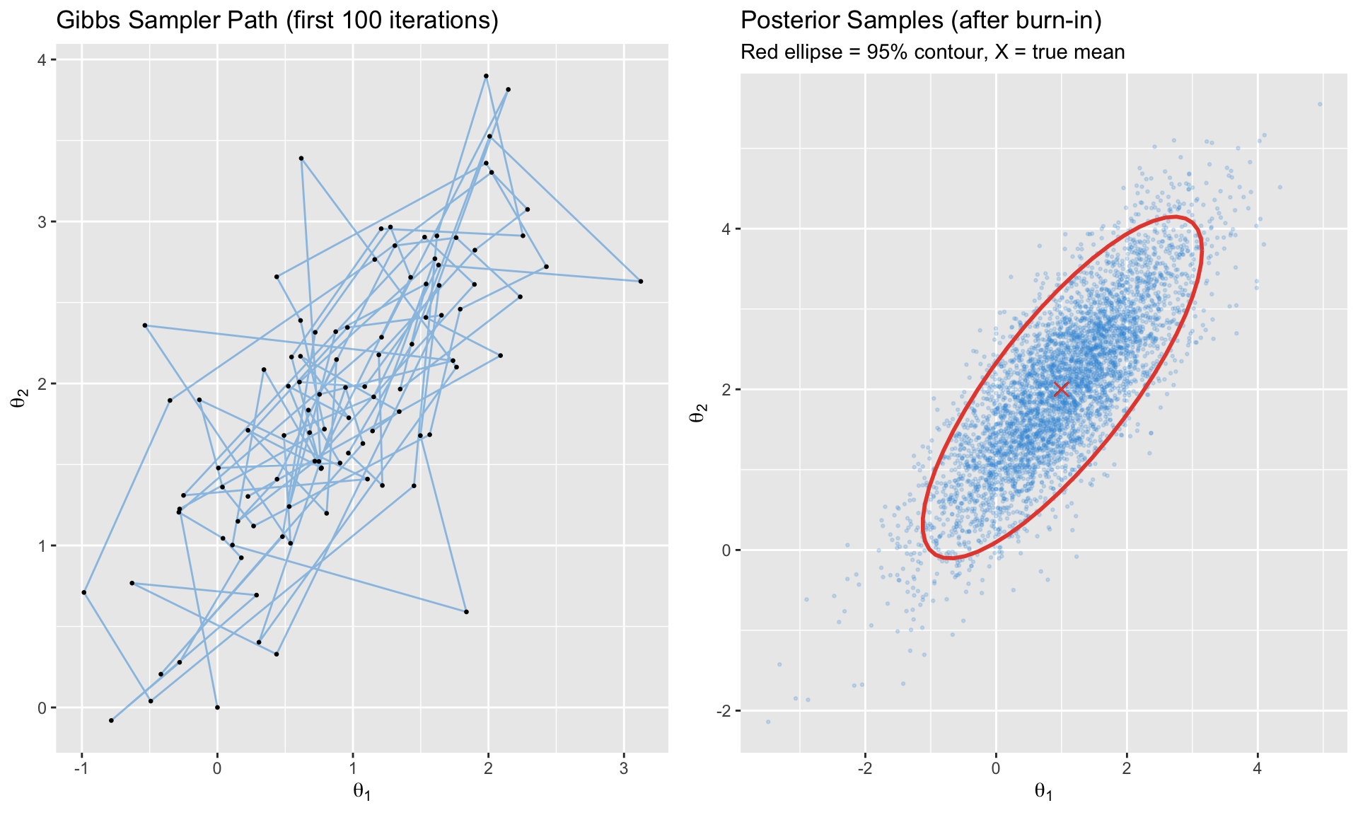
# First 100 iterations showing path
p1 <- ggplot(gibbs_df[1:100, ], aes(x = x1, y = x2)) +
  geom_path(alpha = 0.5, color = "#3498db") +
  geom_point(size = 0.5) +
  labs(title = "Gibbs Sampler Path (first 100 iterations)",
       x = expression(theta[1]), y = expression(theta[2]))

# All samples
p2 <- ggplot(gibbs_df[501:5000, ], aes(x = x1, y = x2)) +
  geom_point(alpha = 0.2, size = 0.5, color = "#3498db") +
  stat_ellipse(level = 0.95, color = "#e74c3c", size = 1) +
  geom_point(aes(x = mu[1], y = mu[2]), color = "#e74c3c", size = 3, shape = 4) +
  labs(title = "Posterior Samples (after burn-in)",
       subtitle = "Red ellipse = 95% contour, X = true mean",
       x = expression(theta[1]), y = expression(theta[2]))

gridExtra::grid.arrange(p1, p2, ncol = 2)

Gibbs sampling from a bivariate normal

Gibbs for Bayesian Regression

For the normal linear model \(Y = X\beta + \varepsilon\) with \(\varepsilon \sim N(0, \sigma^2 I)\):

Block 1: Draw \(\beta | \sigma^2, Y\) \[ \beta | \sigma^2, Y \sim N\left(V_n X'Y, \sigma^2 V_n\right), \quad V_n = (V_0^{-1} + X'X)^{-1} \]

Block 2: Draw \(\sigma^2 | \beta, Y\) \[ \sigma^2 | \beta, Y \sim \text{Inv-Gamma}\left(\frac{\nu_0 + n}{2}, \frac{\nu_0 s_0^2 + (Y-X\beta)'(Y-X\beta)}{2}\right) \]

Hamiltonian Monte Carlo (HMC)

Modern MCMC that uses gradient information for efficient exploration.

Key idea: Treat the parameter space as a physical system. The negative log-posterior is “potential energy.” Add “momentum” variables and simulate Hamiltonian dynamics.

Advantages: - Much more efficient for high-dimensional problems - Fewer iterations needed for convergence - Better exploration of complex posteriors

Implementation: Use Stan (via rstan or cmdstanr) or PyMC

Code
# Comparison table of MCMC methods
mcmc_table <- data.frame(
  Method = c("Metropolis-Hastings", "Gibbs Sampling", "HMC/NUTS"),
  Tuning = c("Proposal variance", "None (if conjugate)", "Step size, path length"),
  Efficiency = c("Low-Medium", "Medium", "High"),
  `Best For` = c("Simple models, low dimensions",
                 "Conjugate models, block structure",
                 "High dimensions, complex posteriors"),
  Software = c("Manual, MCMCpack", "Manual, JAGS", "Stan, PyMC")
)

knitr::kable(mcmc_table, caption = "Comparison of MCMC Methods")
Comparison of MCMC Methods
Method Tuning Efficiency Best.For Software
Metropolis-Hastings Proposal variance Low-Medium Simple models, low dimensions Manual, MCMCpack
Gibbs Sampling None (if conjugate) Medium Conjugate models, block structure Manual, JAGS
HMC/NUTS Step size, path length High High dimensions, complex posteriors Stan, PyMC

Convergence Diagnostics

MCMC is only useful if the chain has converged to the posterior. Always check!

Visual Diagnostics

Trace Plots

The chain should look like a “fuzzy caterpillar”—no trends, quick mixing.

Code
# Good chain
good_chain <- cumsum(rnorm(2000, 0, 1)) * 0.02 + rnorm(2000, 2, 0.5)

# Bad chain (slow mixing)
bad_chain <- numeric(2000)
bad_chain[1] <- -3
for (i in 2:2000) {
  bad_chain[i] <- 0.995 * bad_chain[i-1] + rnorm(1, 0.01, 0.1)
}

trace_comparison <- data.frame(
  iteration = rep(1:2000, 2),
  value = c(good_chain, bad_chain),
  chain = rep(c("Good: Fast Mixing", "Bad: Slow Mixing"), each = 2000)
)

ggplot(trace_comparison, aes(x = iteration, y = value)) +
  geom_line(alpha = 0.7, color = "#3498db") +
  facet_wrap(~chain, scales = "free_y", ncol = 1) +
  labs(title = "Trace Plot Diagnostics",
       subtitle = "Good chains look like 'fuzzy caterpillars'; bad chains show trends or slow drift",
       x = "Iteration", y = expression(theta))

Good vs. bad trace plots

Autocorrelation Plots

Samples should be approximately independent. High autocorrelation = inefficient sampling.

Code
# Calculate ACF
acf_good <- acf(good_chain, lag.max = 50, plot = FALSE)
acf_bad <- acf(bad_chain, lag.max = 50, plot = FALSE)

acf_df <- data.frame(
  lag = rep(0:50, 2),
  acf = c(acf_good$acf, acf_bad$acf),
  chain = rep(c("Good Chain", "Bad Chain"), each = 51)
)

ggplot(acf_df, aes(x = lag, y = acf)) +
  geom_col(fill = "#3498db", width = 0.7) +
  geom_hline(yintercept = c(-0.1, 0.1), linetype = "dashed", color = "#e74c3c") +
  facet_wrap(~chain, ncol = 2) +
  labs(title = "Autocorrelation Function",
       subtitle = "Good chains: ACF drops quickly; Bad chains: ACF stays high",
       x = "Lag", y = "Autocorrelation")

Autocorrelation should decay quickly

Quantitative Diagnostics

Gelman-Rubin \(\hat{R}\) Statistic

Run multiple chains from different starting points. Compare within-chain variance to between-chain variance.

\[ \hat{R} = \sqrt{\frac{\text{Var}(\theta | Y)_{\text{estimate}}}{\text{Within-chain variance}}} \]

Rule: \(\hat{R} < 1.1\) (ideally \(< 1.05\))

Effective Sample Size (ESS)

Accounts for autocorrelation. With \(G\) draws and autocorrelation \(\rho_k\) at lag \(k\):

\[ \text{ESS} = \frac{G}{1 + 2\sum_{k=1}^{\infty} \rho_k} \]

Rule: ESS \(> 400\) for reliable posterior summaries

Code
# Calculate ESS (simplified)
calculate_ess <- function(chain) {
  n <- length(chain)
  acf_vals <- acf(chain, lag.max = min(n-1, 100), plot = FALSE)$acf[-1]

  # Sum until first negative autocorrelation
  sum_rho <- 0
  for (rho in acf_vals) {
    if (rho < 0) break
    sum_rho <- sum_rho + rho
  }

  n / (1 + 2 * sum_rho)
}

cat("Good chain ESS:", round(calculate_ess(good_chain)), "out of", length(good_chain), "\n")
Good chain ESS: 35 out of 2000 
Code
cat("Bad chain ESS:", round(calculate_ess(bad_chain)), "out of", length(bad_chain), "\n")
Bad chain ESS: 14 out of 2000 

Diagnostic Summary Table

Code
diagnostic_table <- data.frame(
  Diagnostic = c("Trace plot", "R-hat", "ESS", "Geweke", "Autocorrelation"),
  Target = c("No trends, good mixing", "< 1.1 (ideally < 1.05)",
             "> 400", "p > 0.05", "Quick decay"),
  `What It Catches` = c("Non-stationarity", "Between-chain disagreement",
                        "High autocorrelation", "Drift in mean",
                        "Inefficient sampling")
)

knitr::kable(diagnostic_table, caption = "MCMC Convergence Diagnostics")
MCMC Convergence Diagnostics
Diagnostic Target What.It.Catches
Trace plot No trends, good mixing Non-stationarity
R-hat < 1.1 (ideally < 1.05) Between-chain disagreement
ESS > 400 High autocorrelation
Geweke p > 0.05 Drift in mean
Autocorrelation Quick decay Inefficient sampling

Model Comparison

Bayesian model comparison answers: “Which model is better supported by the data?”

Marginal Likelihood

The probability of the data under the model:

\[ p(Y | M) = \int p(Y | \theta, M) p(\theta | M) d\theta \]

This is the denominator in Bayes’ theorem—it averages the likelihood over the prior.

Bayes Factors

Compare two models:

\[ BF_{12} = \frac{p(Y | M_1)}{p(Y | M_2)} \]

log(BF) Interpretation
0-1 Not worth mentioning
1-3 Positive evidence
3-5 Strong evidence
> 5 Very strong evidence

Computing Marginal Likelihood

Challenge: The integral is often intractable.

Methods:

  1. Analytical (for conjugate models like NIW-BVAR)
  2. Harmonic Mean (easy but unreliable—avoid!)
  3. Chib’s Method (for Gibbs samplers)
  4. Bridge Sampling (general, reliable)
Code
# Simple example: comparing models with different priors
# Model 1: Tight prior (N(0, 0.5))
# Model 2: Vague prior (N(0, 5))

# For normal-normal model, marginal likelihood is available analytically
# p(Y | prior) = N(Y | prior_mean, prior_var + data_var/n)

y_obs <- c(1.2, 1.5, 0.8, 1.1, 1.4)  # sample data
n <- length(y_obs)
y_bar <- mean(y_obs)
sigma2 <- 1  # known variance

# Marginal likelihood under each prior
log_ml <- function(prior_mean, prior_var, y_bar, n, sigma2) {
  marginal_var <- prior_var + sigma2/n
  dnorm(y_bar, prior_mean, sqrt(marginal_var), log = TRUE)
}

models <- data.frame(
  model = c("M1: Tight prior N(0, 0.5)", "M2: Vague prior N(0, 5)",
            "M3: Centered prior N(1, 1)"),
  prior_mean = c(0, 0, 1),
  prior_var = c(0.5, 5, 1)
)

models$log_ml <- mapply(log_ml, models$prior_mean, models$prior_var,
                        MoreArgs = list(y_bar = y_bar, n = n, sigma2 = sigma2))
models$posterior_prob <- exp(models$log_ml) / sum(exp(models$log_ml))

# Bayes factors relative to M1
models$BF_vs_M1 <- exp(models$log_ml - models$log_ml[1])

cat("Data: y_bar =", round(y_bar, 2), "\n\n")
Data: y_bar = 1.2 
Code
print(models[, c("model", "log_ml", "BF_vs_M1", "posterior_prob")])
                       model    log_ml  BF_vs_M1 posterior_prob
1  M1: Tight prior N(0, 0.5) -1.769172 1.0000000      0.2503422
2    M2: Vague prior N(0, 5) -1.881729 0.8935465      0.2236924
3 M3: Centered prior N(1, 1) -1.026766 2.1009855      0.5259654

Information Criteria

DIC (Deviance Information Criterion): \[ DIC = \bar{D}(\theta) + p_D \] where \(\bar{D}\) is average deviance and \(p_D\) is effective number of parameters.

WAIC (Widely Applicable IC): - Fully Bayesian - Asymptotically equivalent to leave-one-out cross-validation - More reliable than DIC

Rule: Lower is better (like AIC/BIC)

Practical Implementation

R: Using coda for Diagnostics

Code
library(coda)

# Convert MCMC output to coda object
mcmc_chain <- as.mcmc(posterior_draws)

# Diagnostics
plot(mcmc_chain)                    # Trace and density
autocorr.plot(mcmc_chain)           # ACF
effectiveSize(mcmc_chain)           # ESS
geweke.diag(mcmc_chain)             # Geweke test

# For multiple chains
mcmc_list <- mcmc.list(chain1, chain2, chain3)
gelman.diag(mcmc_list)              # R-hat
gelman.plot(mcmc_list)              # R-hat over iterations

R: Using BVAR Package

Code
library(BVAR)

# Estimate Bayesian VAR with Minnesota prior
bvar_model <- bvar(
  data = macro_data,
  lags = 4,
  n_draw = 20000,
  n_burn = 5000,
  priors = bv_minnesota(
    lambda = bv_lambda(mode = 0.2, sd = 0.4, min = 0.0001, max = 5),
    alpha = bv_alpha(mode = 2)
  )
)

# Check convergence
plot(bvar_model)  # trace plots

# Posterior summaries
summary(bvar_model)

# IRFs with credible bands
irf_results <- irf(bvar_model, horizon = 20)
plot(irf_results)

Python: Using PyMC

import pymc as pm
import numpy as np
import arviz as az

# Example: Bayesian linear regression
with pm.Model() as model:
    # Priors
    alpha = pm.Normal("alpha", mu=0, sigma=10)
    beta = pm.Normal("beta", mu=0, sigma=10)
    sigma = pm.HalfNormal("sigma", sigma=1)

    # Likelihood
    mu = alpha + beta * X
    y_obs = pm.Normal("y", mu=mu, sigma=sigma, observed=y)

    # Sample
    trace = pm.sample(2000, tune=1000, cores=2)

# Diagnostics
az.plot_trace(trace)
az.summary(trace)
az.plot_posterior(trace)

# Model comparison
az.waic(trace)
az.loo(trace)

Summary

Key takeaways from this module:

  1. Bayesian inference combines prior beliefs with data through Bayes’ theorem: Posterior ∝ Likelihood × Prior

  2. Why Bayesian for macro:

    • Small samples → priors prevent overfitting
    • Prior information → formally incorporated
    • Full uncertainty quantification → credible intervals
  3. Conjugate priors allow analytical posteriors (Normal-Inverse-Wishart for VARs)

  4. MCMC methods sample from posteriors when analytical solutions don’t exist:

    • Metropolis-Hastings: general purpose
    • Gibbs sampling: for conditional sampling
    • HMC/NUTS: efficient for high dimensions (Stan, PyMC)
  5. Always check convergence:

    • Trace plots (fuzzy caterpillar)
    • R-hat < 1.1
    • ESS > 400
  6. Model comparison via marginal likelihood, Bayes factors, or information criteria (DIC, WAIC)


Key References

Foundational:

  • Koop (2003). Bayesian Econometrics
  • Greenberg (2008). Introduction to Bayesian Econometrics
  • Gelman et al. (2013). Bayesian Data Analysis (3rd ed.)

MCMC Methods:

  • Chib & Greenberg (1995). “Understanding the Metropolis-Hastings Algorithm.” The American Statistician
  • Gelfand & Smith (1990). “Sampling-Based Approaches to Calculating Marginal Densities.” JASA

Diagnostics:

  • Gelman & Rubin (1992). “Inference from Iterative Simulation Using Multiple Sequences.” Statistical Science
  • Vehtari et al. (2021). “Rank-Normalization, Folding, and Localization: An Improved R-hat.” Bayesian Analysis

Model Comparison:

  • Kass & Raftery (1995). “Bayes Factors.” JASA
  • Chib (1995). “Marginal Likelihood from the Gibbs Output.” JASA

Software:


Next: Module 8: Bayesian VARs