Bayesian Panel Methods

Hierarchical Models, Panel VARs, and Cross-Sectional Dependence

The Panel Data Challenge

Cross-country macroeconomic panels present a fundamental tension:

Heterogeneity: Countries differ in institutions, structures, and responses Limited Data: Each country has finite time series (T = 84 quarters) Efficiency: Ignoring cross-country information wastes data

The Core Question

How do we pool information across countries while respecting heterogeneity?

Three Approaches

Approach	Assumption	Problem
Pooled	All countries identical	Ignores heterogeneity
Country-by-country	Countries unrelated	Inefficient, noisy
Hierarchical Bayes	Countries related but different	Best of both worlds

With N = 46 countries and T = 84 quarters, hierarchical Bayesian methods offer the natural solution.

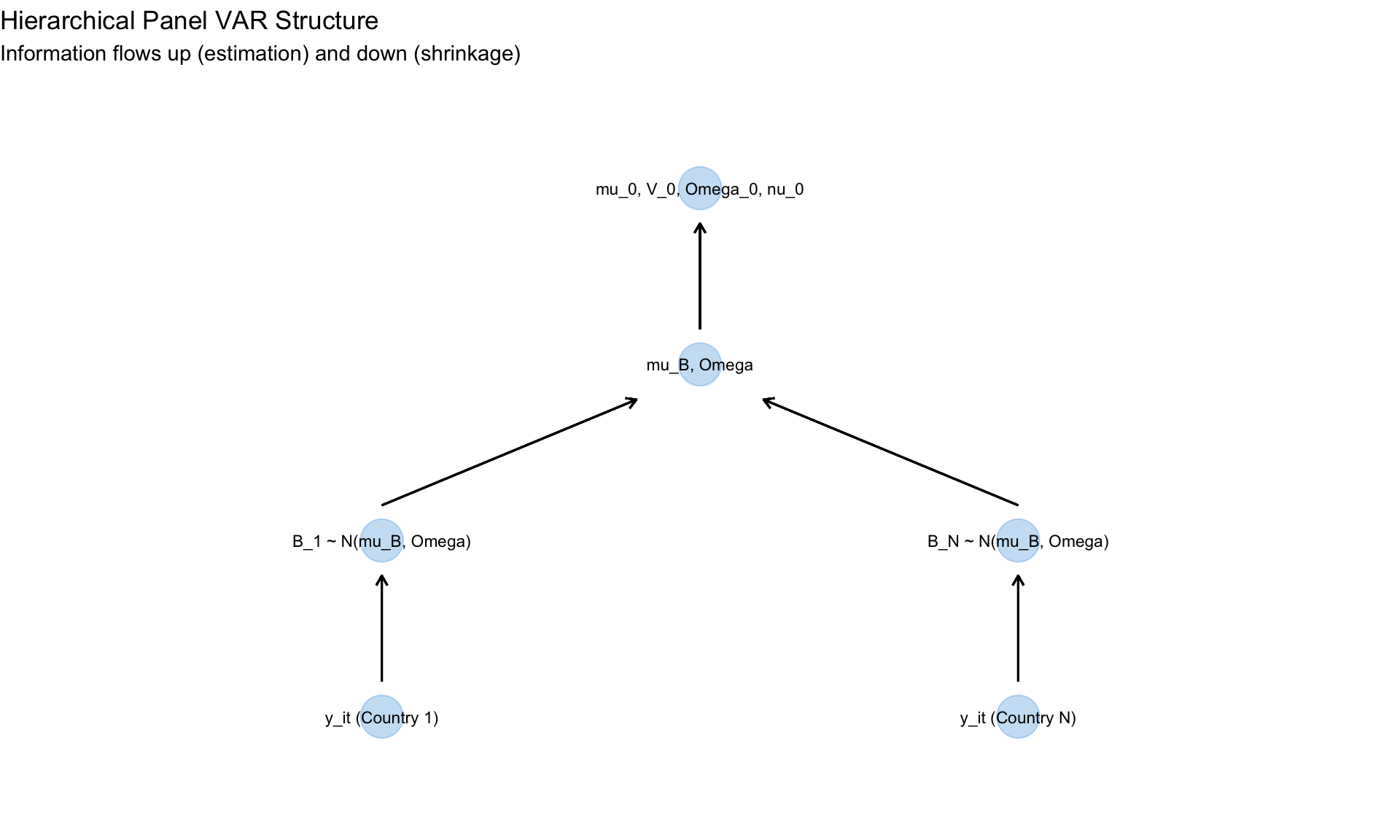
Hierarchical Models: The Framework

The Multilevel Structure

Consider a simple panel regression: \[ y_{it} = x_{it}'\beta_i + \varepsilon_{it}, \quad \varepsilon_{it} \sim N(0, \sigma^2_i) \]

Level 1 (Within-Country): \[ \beta_i | \mu, \Omega \sim N(\mu, \Omega) \]

Level 2 (Across-Countries): \[ \mu \sim N(\mu_0, V_0), \quad \Omega \sim \text{Inverse-Wishart}(\Omega_0, \nu_0) \]

The country-specific coefficients \(\beta_i\) are drawn from a common distribution with unknown mean \(\mu\) and variance \(\Omega\).

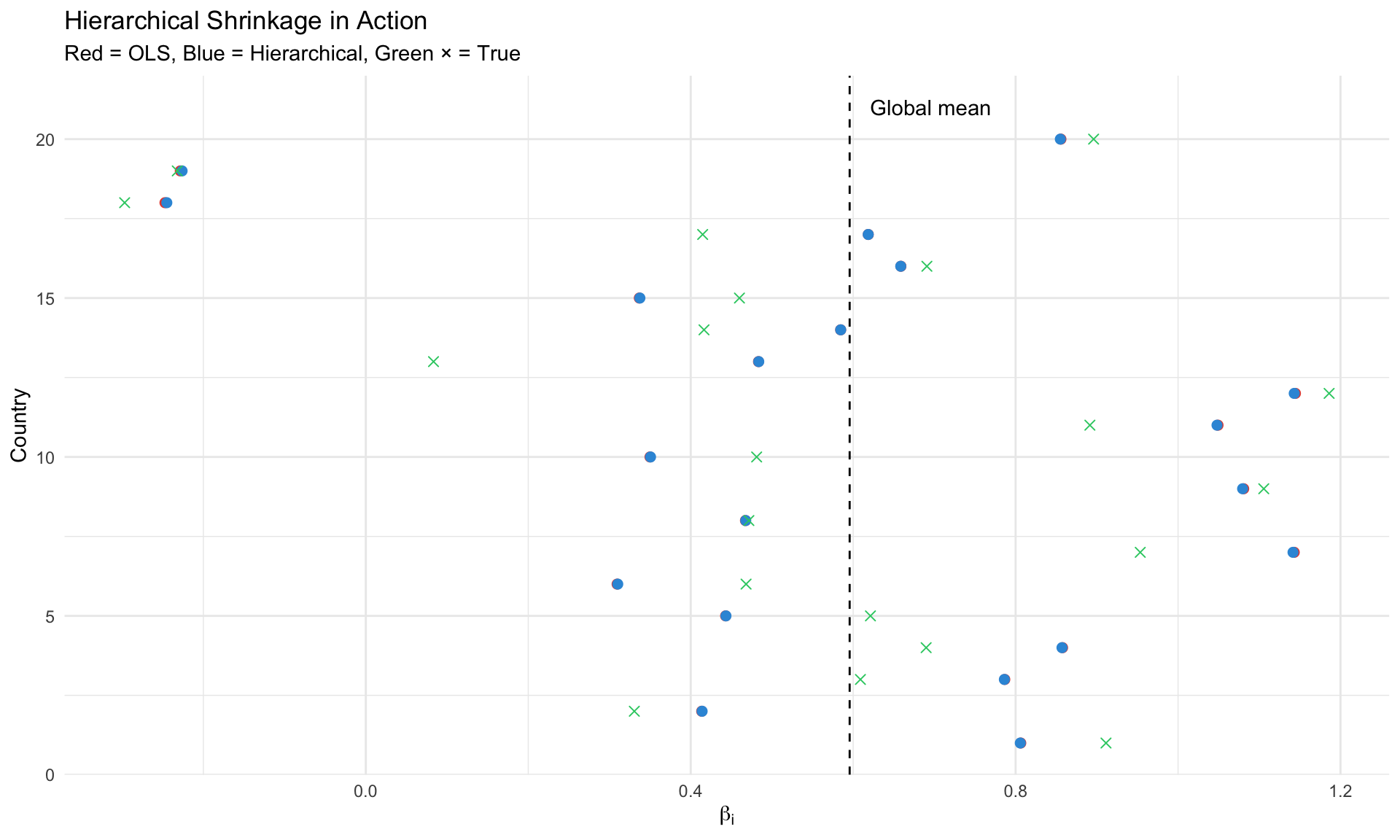
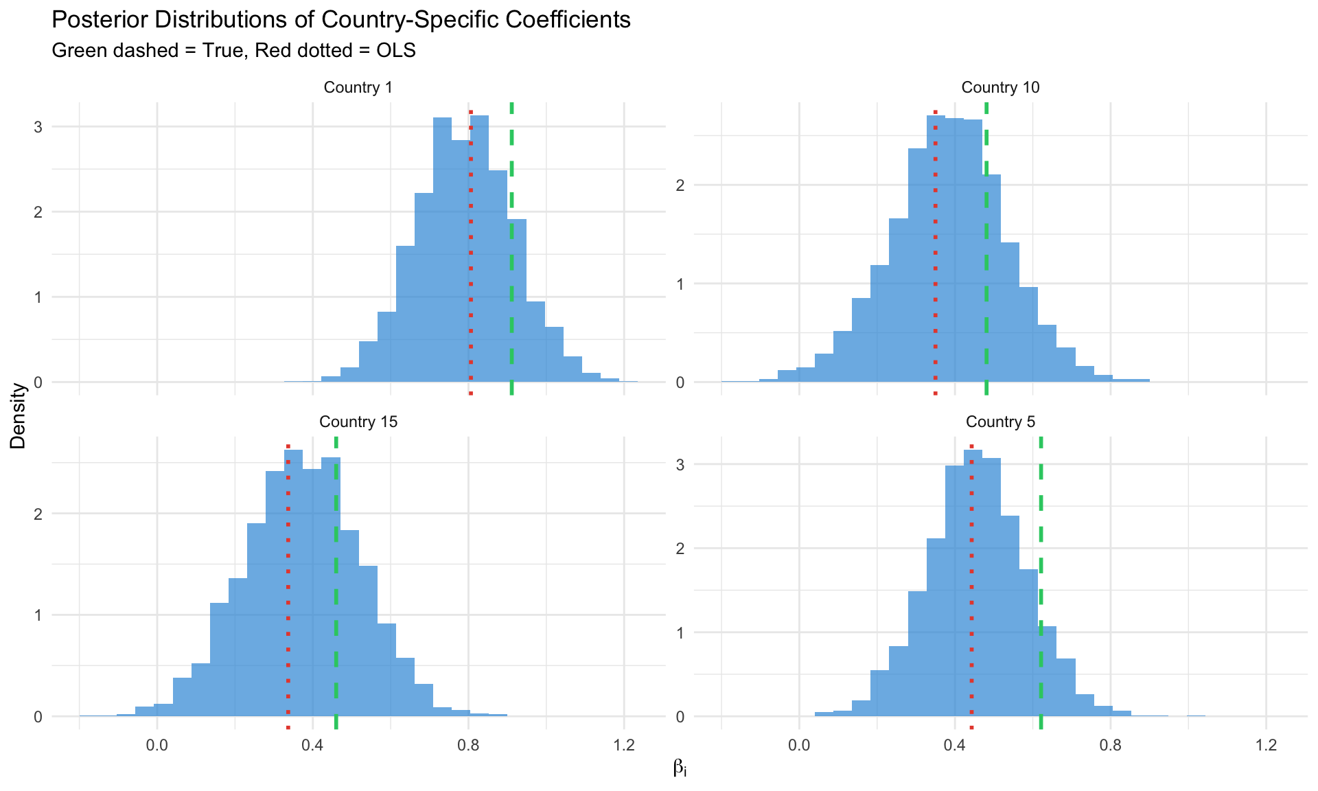
Shrinkage and Partial Pooling

The posterior for \(\beta_i\) combines:

Country-specific data (likelihood)
Cross-country information (hierarchical prior)

\[ \hat{\beta}_i^{\text{Bayes}} = \lambda_i \hat{\beta}_i^{\text{OLS}} + (1 - \lambda_i) \bar{\beta} \]

where \(\lambda_i \in [0,1]\) depends on: - Precision of country data: More data → less shrinkage - Cross-country heterogeneity: More variance in \(\Omega\) → less shrinkage

Hierarchical shrinkage: country estimates pulled toward global mean

Why Shrinkage Helps

Key Insight: Countries with less precise estimates get shrunk more toward the global mean.

Country Type	Data Quality	Shrinkage	Result
Data-rich (US, Germany)	High	Low	Near OLS
Data-poor (small EMs)	Low	High	Near global mean

This is not bias — it’s optimal use of information under the hierarchical structure.

Gibbs Sampler for Hierarchical Panel

The Algorithm

For the hierarchical linear model:

Block 1: Draw \(\beta_i | y_i, \mu, \Omega, \sigma^2_i\) for each country \[ \beta_i | \cdot \sim N\left( V_i^{-1}(X_i'y_i/\sigma^2_i + \Omega^{-1}\mu), V_i^{-1} \right) \] where \(V_i = X_i'X_i/\sigma^2_i + \Omega^{-1}\)

Block 2: Draw \(\sigma^2_i | y_i, \beta_i\) \[ \sigma^2_i | \cdot \sim \text{Inverse-Gamma}\left( \frac{T_i}{2}, \frac{(y_i - X_i\beta_i)'(y_i - X_i\beta_i)}{2} \right) \]

Block 3: Draw \(\mu | \beta_1, \ldots, \beta_N, \Omega\) \[ \mu | \cdot \sim N\left( (N\Omega^{-1} + V_0^{-1})^{-1}(N\Omega^{-1}\bar{\beta} + V_0^{-1}\mu_0), (N\Omega^{-1} + V_0^{-1})^{-1} \right) \]

Block 4: Draw \(\Omega | \beta_1, \ldots, \beta_N, \mu\) \[ \Omega | \cdot \sim \text{Inverse-Wishart}\left( \Omega_0 + \sum_{i=1}^N (\beta_i - \mu)(\beta_i - \mu)', \nu_0 + N \right) \]

Posterior distributions from hierarchical panel model

Bayesian Panel VAR

The Model Structure

For N countries, each with a K-variable VAR(p):

\[ y_{it} = c_i + A_{i,1} y_{i,t-1} + \cdots + A_{i,p} y_{i,t-p} + u_{it} \]

Hierarchical Prior: \[ \text{vec}(B_i) | \mu_B, \Omega_B \sim N(\mu_B, \Omega_B) \]

where \(B_i = [c_i, A_{i,1}, \ldots, A_{i,p}]'\) stacks all VAR coefficients for country \(i\).

Why Panel VAR?

Feature	Separate VARs	Pooled VAR	Panel VAR
Heterogeneity	Yes	No	Yes
Sample size	T per country	N×T	N×T (shared info)
Curse of dimensionality	Severe	Moderate	Mitigated
Interpretation	Country-specific	Global average	Both

With K = 3 variables, p = 2 lags, and T = 84: - Parameters per country: 3 × (1 + 3×2) = 21 - Observations per country: 84 - 2 = 82 - Degrees of freedom: Tight!

Hierarchical pooling provides effective sample size boost without forcing homogeneity.

Mean-Group Prior Structure

Following Canova & Ciccarelli (2009), we can decompose:

\[ B_i = \underbrace{\bar{B}}_{\text{common}} + \underbrace{\tilde{B}_i}_{\text{country-specific}} + \underbrace{Z_i \gamma}_{\text{observed heterogeneity}} \]

where: - \(\bar{B}\): Common component (global dynamics) - \(\tilde{B}_i\): Idiosyncratic deviation - \(Z_i\): Country characteristics (GDP per capita, openness, institutions)

Panel VAR structure for cross-country macro analysis

Gibbs Sampler for Panel VAR

Estimating Panel VAR...

Draw 500 of 2500 
Draw 1000 of 2500 
Draw 1500 of 2500 
Draw 2000 of 2500 
Draw 2500 of 2500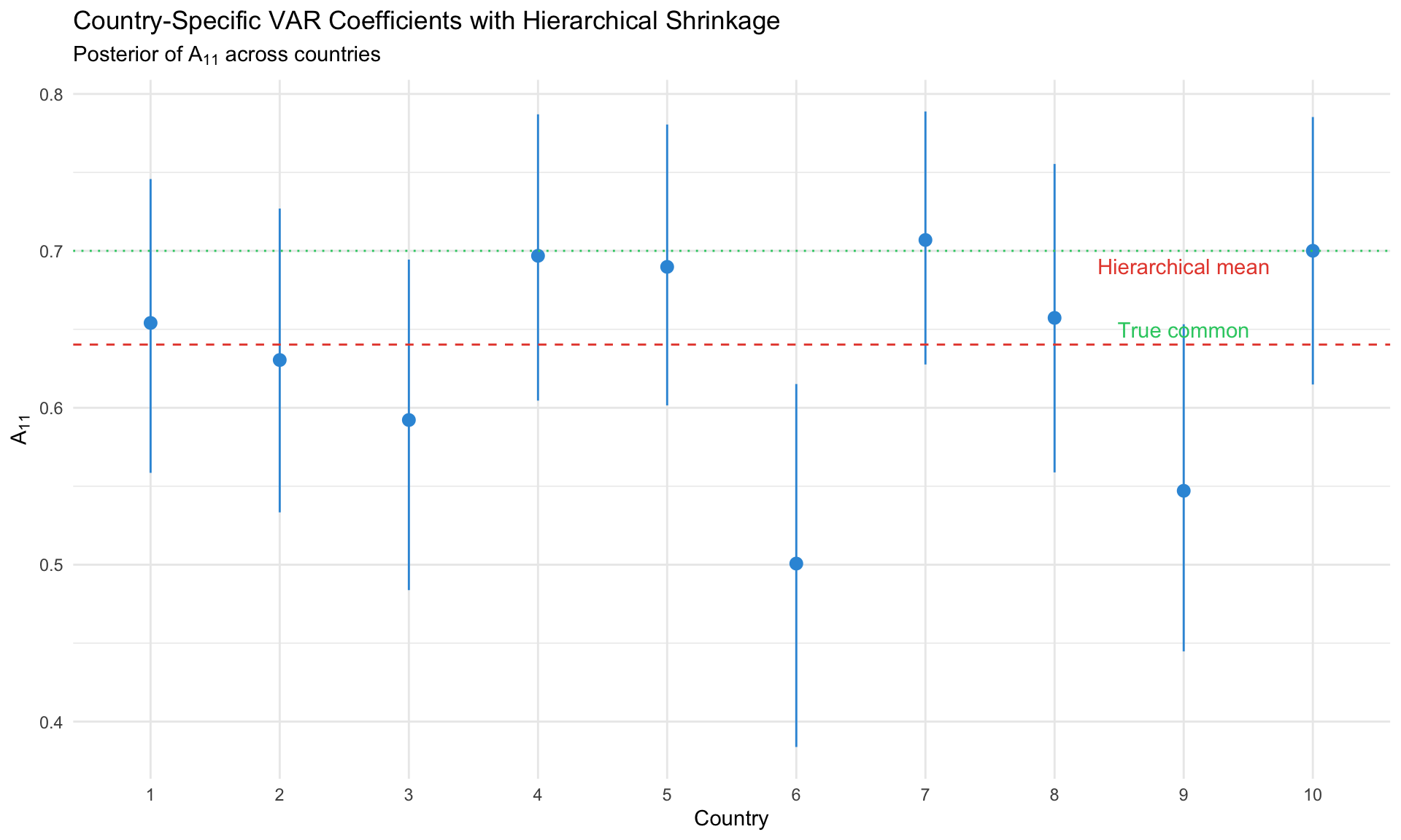

Panel VAR coefficient posteriors across countries

Random Coefficients Models

Swamy (1970) Random Coefficients

The classic frequentist approach:

\[ y_{it} = x_{it}'\beta_i + \varepsilon_{it} \] \[ \beta_i = \bar{\beta} + v_i, \quad v_i \sim N(0, \Omega) \]

Bayesian version adds priors on \((\bar{\beta}, \Omega)\) and uses Gibbs sampling.

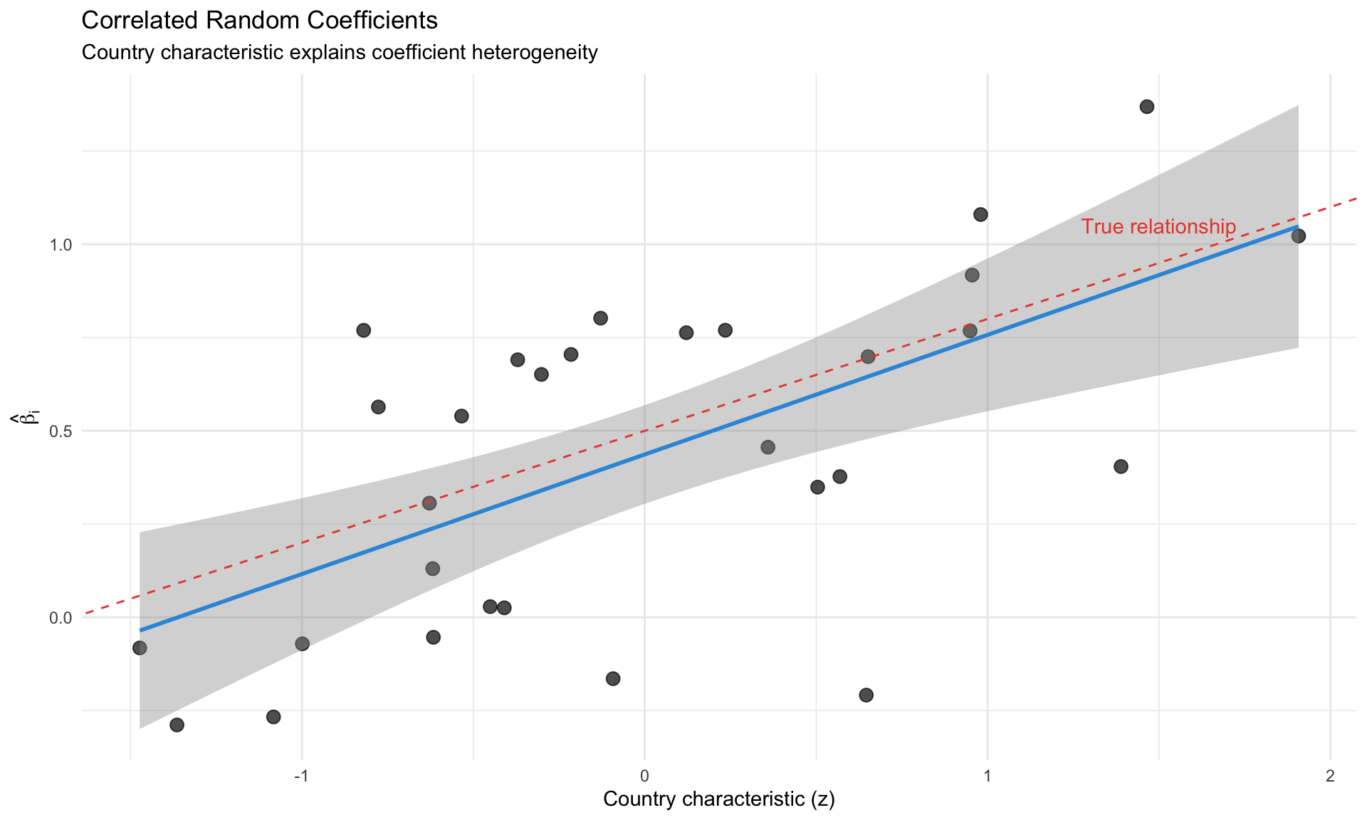
Correlated Random Coefficients

Allow \(\beta_i\) to correlate with observables:

\[ \beta_i = \bar{\beta} + Z_i'\gamma + v_i \]

where \(Z_i\) are country characteristics (GDP per capita, openness, institutions).

Application: Countries with higher institutional quality might have different Taylor rule coefficients.

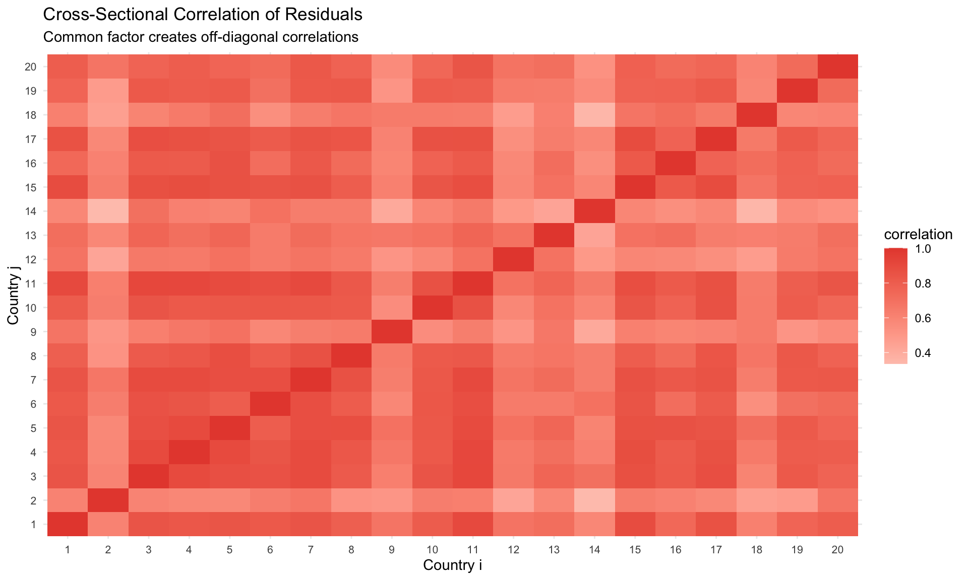
Random coefficients with observable heterogeneity

Cross-Sectional Dependence

The Problem

Standard panel methods assume: \[ E[\varepsilon_{it} \varepsilon_{js}] = 0 \quad \text{for } i \neq j \]

But in macro panels, global shocks (oil prices, US monetary policy, COVID) create cross-sectional dependence.

Factor Structure Approach

Model the error as: \[ \varepsilon_{it} = \lambda_i' f_t + e_{it} \]

where: - \(f_t\): Common factors (K_f × 1) - \(\lambda_i\): Country-specific factor loadings - \(e_{it}\): Idiosyncratic error

Interactive Fixed Effects (Bai 2009)

\[ y_{it} = x_{it}'\beta + \lambda_i' f_t + e_{it} \]

Jointly estimates \(\beta\), \(\Lambda = [\lambda_1, \ldots, \lambda_N]'\), and \(F = [f_1, \ldots, f_T]'\).

Bayesian Factor Model

Prior structure: \[ f_t | \Sigma_f \sim N(0, \Sigma_f), \quad \lambda_i \sim N(0, \Omega_\lambda) \]

Identification: Impose lower-triangular structure on loadings (first K_f countries).

Cross-sectional dependence via common factor

Bayesian Factor-Augmented Panel VAR

Combine hierarchical panel VAR with factor structure:

\[ y_{it} = c_i + A_i y_{i,t-1} + \Gamma_i f_t + u_{it} \]

where \(f_t\) is a vector of global factors (extracted or observed).

Application in macro: Include Global Financial Cycle (GFC) factor from Miranda-Agrippino & Rey.

Python Implementation

For larger panels or more complex hierarchical structures, Python with NumPy/SciPy provides flexibility.

# Hierarchical Panel Model in Python
import numpy as np
from scipy import stats
from scipy.linalg import solve, cholesky

def hierarchical_panel_gibbs(y_list, X_list, n_draw=5000, n_burn=1000):
    """
    Gibbs sampler for hierarchical panel regression.

    y_list: list of (T_i,) arrays - outcomes by country
    X_list: list of (T_i, K) arrays - regressors by country
    """
    N = len(y_list)
    K = X_list[0].shape[1]

    # Priors
    mu0 = np.zeros(K)
    V0 = np.eye(K) * 10
    V0_inv = np.linalg.inv(V0)
    Omega0 = np.eye(K)
    nu0 = K + 2
    a0, b0 = 0.01, 0.01  # for sigma^2

    # Storage
    beta_draws = np.zeros((n_draw, N, K))
    mu_draws = np.zeros((n_draw, K))
    Omega_draws = np.zeros((n_draw, K, K))

    # Initialize
    beta_curr = np.zeros((N, K))
    for i in range(N):
        beta_curr[i] = np.linalg.lstsq(X_list[i], y_list[i], rcond=None)[0]
    sigma2_curr = np.ones(N)
    mu_curr = beta_curr.mean(axis=0)
    Omega_curr = np.cov(beta_curr.T) + 0.01 * np.eye(K)

    for g in range(n_draw + n_burn):
        Omega_inv = np.linalg.inv(Omega_curr)

        # Block 1: Draw beta_i | rest
        for i in range(N):
            X_i, y_i = X_list[i], y_list[i]
            XtX = X_i.T @ X_i
            Xty = X_i.T @ y_i

            V_post_inv = XtX / sigma2_curr[i] + Omega_inv
            V_post = np.linalg.inv(V_post_inv)
            m_post = V_post @ (Xty / sigma2_curr[i] + Omega_inv @ mu_curr)

            beta_curr[i] = np.random.multivariate_normal(m_post, V_post)

        # Block 2: Draw sigma2_i | rest
        for i in range(N):
            resid = y_list[i] - X_list[i] @ beta_curr[i]
            T_i = len(y_list[i])
            a_post = a0 + T_i / 2
            b_post = b0 + np.sum(resid**2) / 2
            sigma2_curr[i] = 1 / np.random.gamma(a_post, 1/b_post)

        # Block 3: Draw mu | rest
        V_mu_post = np.linalg.inv(N * Omega_inv + V0_inv)
        m_mu_post = V_mu_post @ (N * Omega_inv @ beta_curr.mean(axis=0) +
                                  V0_inv @ mu0)
        mu_curr = np.random.multivariate_normal(m_mu_post, V_mu_post)

        # Block 4: Draw Omega | rest (Inverse Wishart)
        S_post = Omega0.copy()
        for i in range(N):
            diff = beta_curr[i] - mu_curr
            S_post += np.outer(diff, diff)

        # Draw from Inverse Wishart
        df_post = nu0 + N
        Omega_curr = stats.invwishart.rvs(df=df_post, scale=S_post)

        # Store
        if g >= n_burn:
            idx = g - n_burn
            beta_draws[idx] = beta_curr
            mu_draws[idx] = mu_curr
            Omega_draws[idx] = Omega_curr

    return {
        'beta': beta_draws,
        'mu': mu_draws,
        'Omega': Omega_draws
    }

# Example usage:
# result = hierarchical_panel_gibbs(y_list, X_list)
# beta_posterior_mean = result['beta'].mean(axis=0)

Model Comparison for Panel Models

Marginal Likelihood

For hierarchical models, the marginal likelihood integrates over all parameters:

\[ p(Y | M) = \int p(Y | \theta) p(\theta | M) d\theta \]

For linear hierarchical models: Often tractable analytically.

For complex models: Use bridge sampling or the Chib (1995) method.

DIC and WAIC

Criterion	Formula	Use
DIC	\(\bar{D} + p_D\)	Effective parameters penalty
WAIC	Pointwise predictive density	Better for hierarchical models
LOO-CV	Leave-one-out cross-validation	Gold standard but expensive

DIC: 2873.5

Effective parameters (p_D): 36.9

Practical Guidance

When to Use Hierarchical vs. Standard Panel

Situation	Recommendation
Small T per country (< 30)	Hierarchical (shrinkage helps)
Large N, moderate T	Hierarchical (efficient)
Focus on average effect	Either works
Focus on heterogeneity	Hierarchical (full posterior)
Strong prior beliefs	Bayesian hierarchical

Implementation Checklist

Check MCMC convergence: Trace plots, R-hat, effective sample size
Assess shrinkage: Compare hierarchical to OLS estimates
Test homogeneity: Is \(\Omega\) small relative to coefficient magnitudes?
Cross-sectional dependence: Test residuals, consider factors
Model comparison: DIC/WAIC across specifications

Common Pitfalls

Watch Out For

Over-shrinkage: Very tight hyperpriors force all countries to look identical
Under-shrinkage: Vague hyperpriors fail to borrow strength
Ignoring cross-sectional dependence: Biases standard errors downward
Too many parameters: K-variable panel VAR with p lags has \(N \times K \times (Kp + 1)\) parameters
Improper mixing: Hierarchical models can have slow mixing — increase draws

Key References

Hierarchical Panel Models

Gelman & Hill (2007) Data Analysis Using Regression and Multilevel/Hierarchical Models — Accessible introduction
Swamy (1970) “Efficient Inference in a Random Coefficient Regression Model” Econometrica — Classic random coefficients
Hsiao (2014) Analysis of Panel Data — Comprehensive textbook

Bayesian Panel VAR

Canova & Ciccarelli (2009) “Estimating Multicountry VAR Models” IER — Foundational paper
Canova & Ciccarelli (2013) “Panel Vector Autoregressive Models: A Survey” — Survey chapter
Jarocinski (2010) “Responses to Monetary Policy Shocks in the East and the West of Europe” JAE — Application

Cross-Sectional Dependence

Bai (2009) “Panel Data Models with Interactive Fixed Effects” Econometrica — Factor structure
Pesaran (2006) “Estimation and Inference in Large Heterogeneous Panels” Econometrica — CCE estimator
Chudik & Pesaran (2015) “Common Correlated Effects Estimation of Heterogeneous Dynamic Panel Data Models” JoE

Software

R: brms (Bürkner), lme4 (Bates et al.), custom Gibbs samplers
Python: PyMC, NumPy/SciPy for manual MCMC
Stan: rstan/pystan for complex hierarchical models

Summary

Concept	Key Insight
Hierarchical models	Pool information while allowing heterogeneity
Shrinkage	Data-poor countries borrow from data-rich
Panel VAR	Country-specific dynamics with common structure
Cross-sectional dependence	Global factors create correlations
Gibbs sampling	Natural framework for hierarchical models

For Your Research

With N = 46 countries and T = 84 quarters: - Hierarchical shrinkage is valuable for EM countries with noisier data - Panel VAR can reveal heterogeneity in policy transmission - Factor structures capture global shocks (GFC, COVID) - Always check cross-sectional correlation in residuals