Vector Autoregressions

From Reduced Form to Structural Identification

The VAR Framework

Vector Autoregressions (VARs) model the joint dynamics of multiple time series. VARs became the workhorse of empirical macroeconomics because they impose minimal theoretical structure while capturing rich dynamic interactions. For a comprehensive treatment, see Kilian and Lütkepohl (2017).

From Single Equations to Systems

Consider a simple monetary policy question: How does output respond to an interest rate change?

Single equation approach: \[ y_t = \alpha + \beta \cdot r_t + \varepsilon_t \]

Problems: - Interest rates respond to output (simultaneity) - Past values of both matter (dynamics) - Other variables are omitted

VAR approach: Model everything jointly: \[ \begin{bmatrix} y_t \\ \pi_t \\ r_t \end{bmatrix} = \mathbf{c} + \mathbf{A}_1 \begin{bmatrix} y_{t-1} \\ \pi_{t-1} \\ r_{t-1} \end{bmatrix} + \mathbf{A}_2 \begin{bmatrix} y_{t-2} \\ \pi_{t-2} \\ r_{t-2} \end{bmatrix} + \begin{bmatrix} u_{1t} \\ u_{2t} \\ u_{3t} \end{bmatrix} \]

Reduced-Form VAR

The Model

A VAR(p) for K variables: \[ \mathbf{y}_t = \mathbf{c} + \mathbf{A}_1 \mathbf{y}_{t-1} + \mathbf{A}_2 \mathbf{y}_{t-2} + \cdots + \mathbf{A}_p \mathbf{y}_{t-p} + \mathbf{u}_t \]

where: - \(\mathbf{y}_t\) is \(K \times 1\) vector of endogenous variables - \(\mathbf{A}_j\) are \(K \times K\) coefficient matrices - \(\mathbf{u}_t \sim N(\mathbf{0}, \boldsymbol{\Sigma}_u)\) are reduced-form residuals - \(\boldsymbol{\Sigma}_u\) captures contemporaneous correlations

Key property: Reduced-form residuals \(\mathbf{u}_t\) are correlated across equations. They are not structural shocks.

Estimation

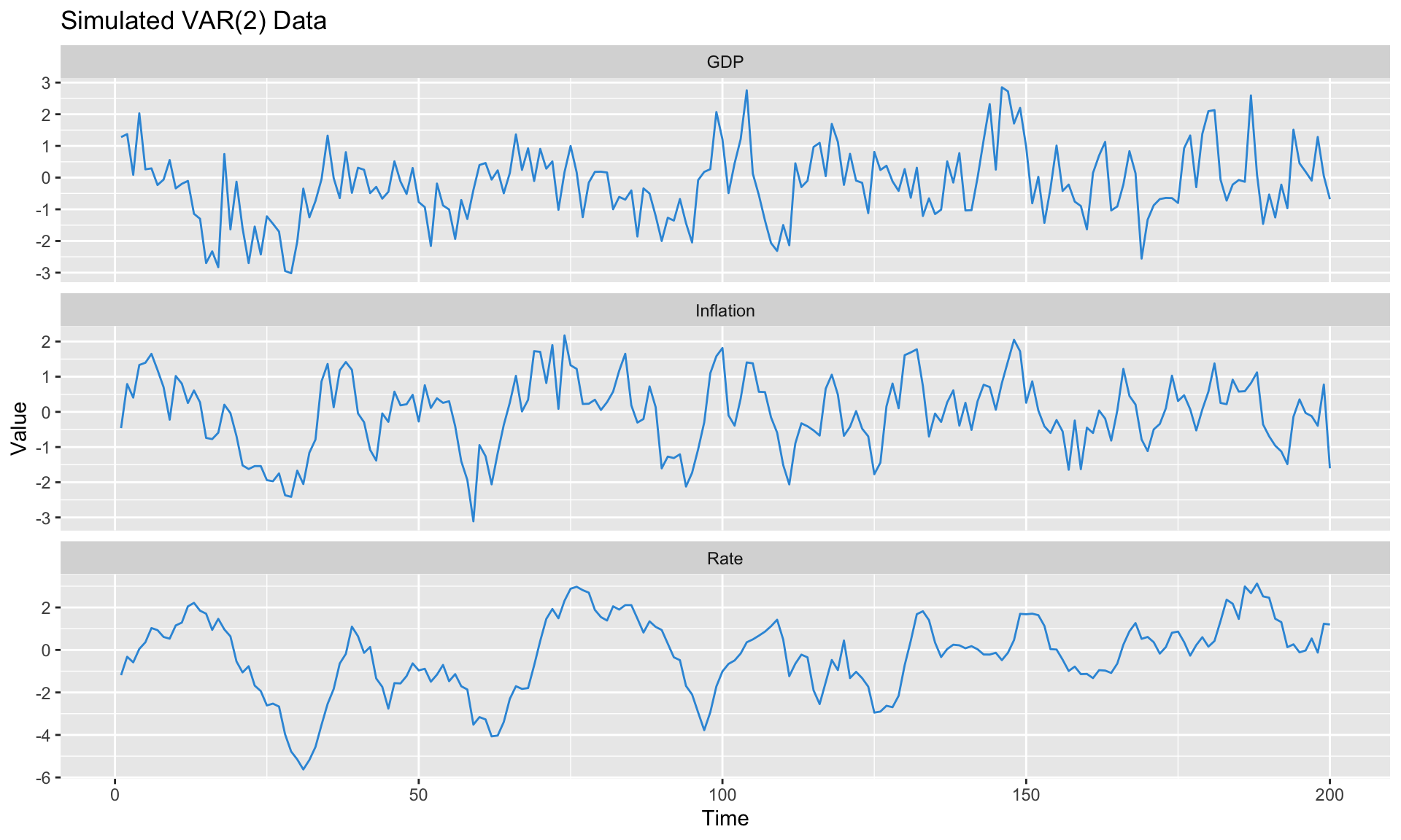
Each equation can be estimated by OLS (since all equations have the same regressors). Let’s simulate and estimate.

Lag selection criteria:

AIC(n)  HQ(n)  SC(n) FPE(n) 
     2      1      1      2


Eigenvalues of companion matrix (all should be < 1):

[1] 0.838 0.838 0.639 0.371 0.123 0.123

Companion Form and Stability

For analysis, we write the VAR in companion form: \[ \mathbf{Y}_t = \mathbf{A}_{comp} \mathbf{Y}_{t-1} + \mathbf{U}_t \]

where \(\mathbf{Y}_t = [\mathbf{y}_t', \mathbf{y}_{t-1}', \ldots]'\) stacks lagged values.

Stability condition: All eigenvalues of \(\mathbf{A}_{comp}\) must lie inside the unit circle. If any eigenvalue equals 1, there’s a unit root; if greater than 1, the system is explosive.

The Identification Problem

Why Structure Matters

The reduced-form VAR gives us \(\boldsymbol{\Sigma}_u\)—the covariance of residuals. But we want structural shocks \(\boldsymbol{\varepsilon}_t\) that are: - Uncorrelated with each other - Have economic interpretation (demand shock, supply shock, monetary shock)

The structural form: \[ \mathbf{B}_0 \mathbf{y}_t = \mathbf{b}_0 + \mathbf{B}_1 \mathbf{y}_{t-1} + \cdots + \boldsymbol{\varepsilon}_t, \quad \boldsymbol{\varepsilon}_t \sim N(\mathbf{0}, \mathbf{I}) \]

Connection to reduced form: \[ \mathbf{u}_t = \mathbf{B}_0^{-1} \boldsymbol{\varepsilon}_t \implies \boldsymbol{\Sigma}_u = \mathbf{B}_0^{-1} (\mathbf{B}_0^{-1})' \]

The Counting Problem

With K variables: - \(\boldsymbol{\Sigma}_u\) has \(K(K+1)/2\) unique elements - \(\mathbf{B}_0^{-1}\) has \(K^2\) elements - We need \(K(K-1)/2\) additional restrictions

For K=3: We observe 6 unique elements of \(\Sigma_u\), but need 9 elements of \(B_0^{-1}\). We need 3 restrictions.

The Fundamental Challenge

Moving from reduced-form to structural requires identifying assumptions. Different assumptions = different structural shocks = potentially different conclusions.

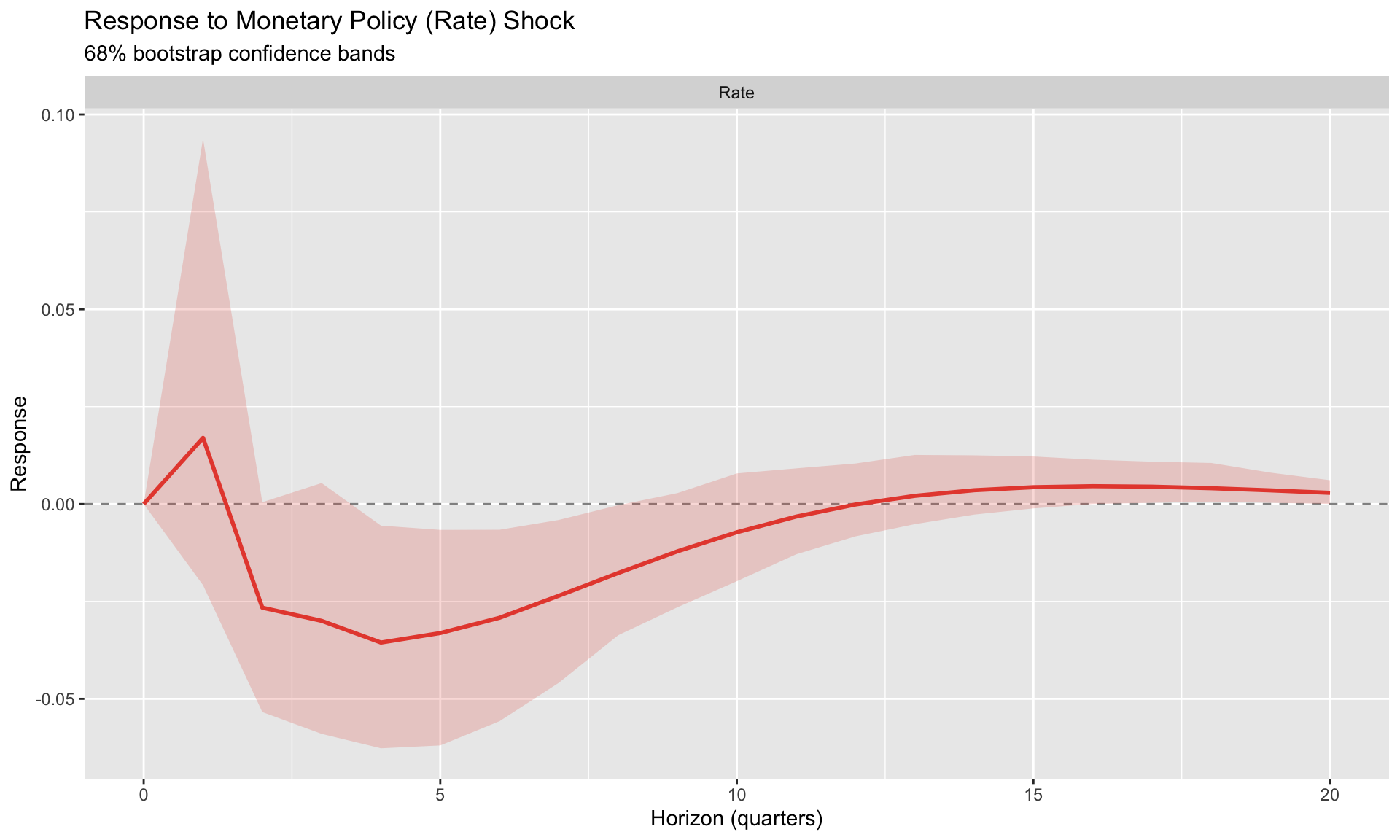
Recursive (Cholesky) Identification

The Approach

The simplest identification: assume a recursive causal ordering.

\[ \mathbf{B}_0^{-1} = \text{chol}(\boldsymbol{\Sigma}_u) \quad \text{(lower triangular)} \]

This imposes: - Variable 1 doesn’t respond contemporaneously to variables 2 or 3 - Variable 2 doesn’t respond contemporaneously to variable 3 - Variable 3 responds to everything

Economic Interpretation

For monetary policy, a common ordering: slow → policy → fast

GDP (slow): doesn’t respond within quarter to anything
Inflation (medium): responds to GDP shocks, not rate within quarter
Interest rate (fast): central bank sees GDP and inflation, then sets rate

Impulse responses to monetary policy shock (Cholesky identification)

The Ordering Problem

Cholesky identification is sensitive to ordering. Let’s see what happens with a different order:

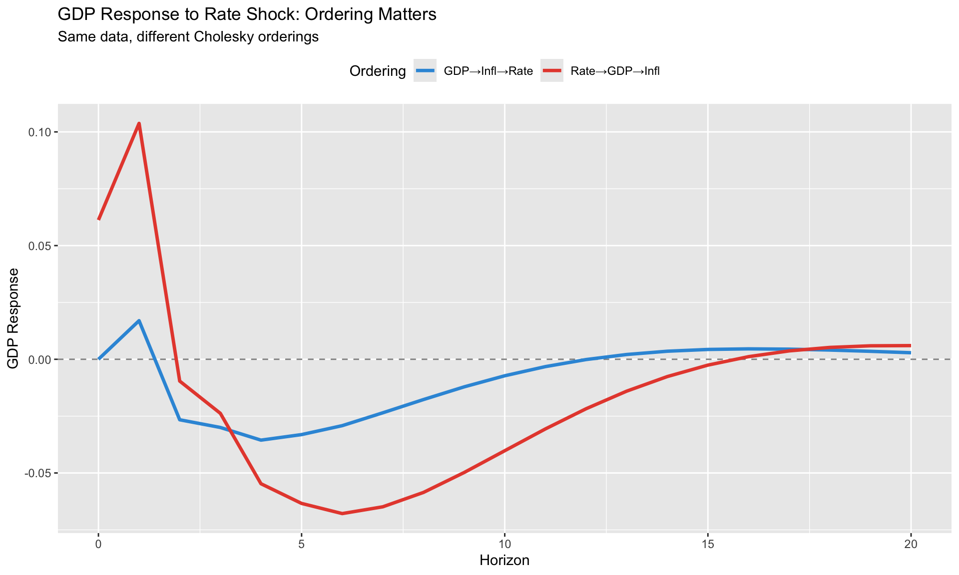
Always Check Robustness

If your conclusions change substantially with ordering, your identification is fragile. Report results under alternative orderings.

Sign Restrictions

The Idea

Instead of exact zero restrictions, impose inequality constraints based on economic theory.

For a monetary policy tightening: - Interest rate rises (+) - Output falls (−) - Inflation falls (−)

This doesn’t uniquely identify the shock—it defines a set of admissible structural models.

Algorithm

Compute any valid \(\mathbf{B}_0^{-1}\) (e.g., Cholesky)
Draw a random orthogonal matrix \(\mathbf{Q}\)
Candidate: \(\tilde{\mathbf{B}} = \mathbf{B}_0^{-1} \mathbf{Q}\)
Compute IRFs with \(\tilde{\mathbf{B}}\)
Check if signs match restrictions
If yes: accept. If no: reject and return to step 2.

Acceptance rate: 24.3 %

Accepted draws: 50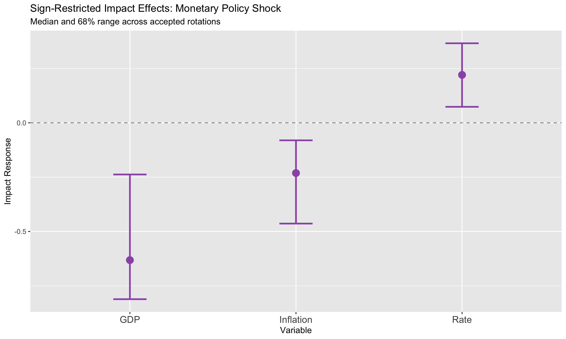

Sign-restricted IRFs show a range of admissible models

Full Implementation

For complete sign-restricted IRFs across all horizons, use the svars package:

library(svars)
id.sign(var_model, restriction_matrix = sign_matrix)

Set Identification vs. Point Identification

Aspect	Point Identification (Cholesky)	Set Identification (Signs)
Result	Single IRF	Range of IRFs
Assumptions	Exact zeros	Inequality constraints
Robustness	Sensitive to ordering	Theory-guided
Interpretation	“The” effect	Bounds on effect

External Instruments (Proxy SVAR)

The Approach

Use an external instrument \(z_t\) correlated with one structural shock but not others.

Requirements: - Relevance: \(E[z_t \varepsilon_{1t}] \neq 0\) - Exogeneity: \(E[z_t \varepsilon_{jt}] = 0\) for \(j \neq 1\)

Common instruments for monetary policy: - High-frequency surprises around FOMC announcements - Narrative identification (Romer & Romer)

Implementation

First-stage F-statistic: 76.05

Estimated impact vector: -0.02 0.292 1

The F-Statistic Rule

A first-stage F-statistic below 10 indicates a weak instrument. Inference becomes unreliable. Always report the F-stat!

Forecast Error Variance Decomposition

The Question

At horizon \(h\), what fraction of the forecast error variance of variable \(i\) is attributable to structural shock \(j\)?

\[ \text{FEVD}_{i,j}(h) = \frac{\sum_{s=0}^{h} (\mathbf{e}_i' \boldsymbol{\Phi}_s \mathbf{B}_0^{-1} \mathbf{e}_j)^2}{\sum_{s=0}^{h} \mathbf{e}_i' \boldsymbol{\Phi}_s \boldsymbol{\Sigma}_u \boldsymbol{\Phi}_s' \mathbf{e}_i} \]

Implementation

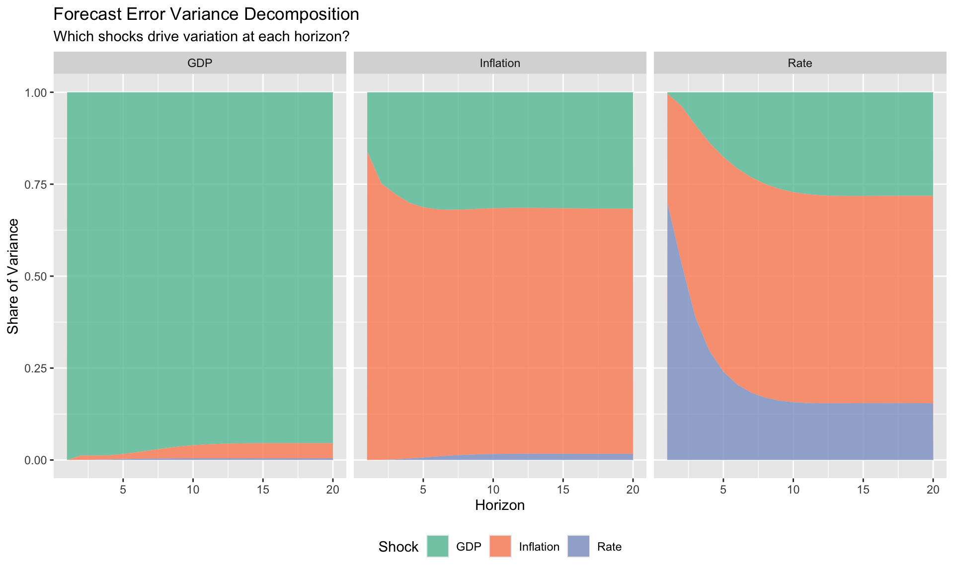
Forecast error variance decomposition over horizons

Interpretation

At short horizons, own shocks typically dominate
As horizons extend, other shocks become relatively more important
At long horizons: reveals which shocks drive permanent movements

Historical Decomposition

The Question

What would the path of variable \(i\) have been if only shock \(j\) had occurred?

\[ y_{it} = \text{deterministic} + \sum_{j=1}^{K} \underbrace{\sum_{s=0}^{t} \Phi_{ij,s} \cdot \varepsilon_{j,t-s}}_{\text{contribution of shock } j} \]

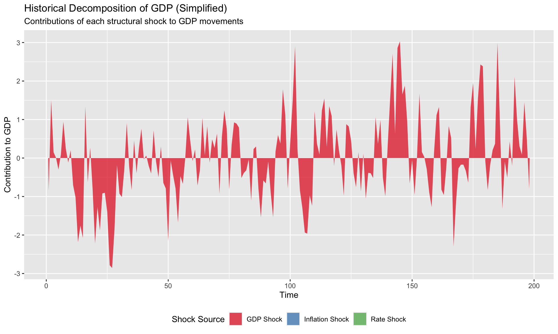
Historical decomposition: contributions of each shock to GDP

Full Historical Decomposition

The vars package provides complete historical decomposition via historical_decomposition(). The simplified version above illustrates the concept.

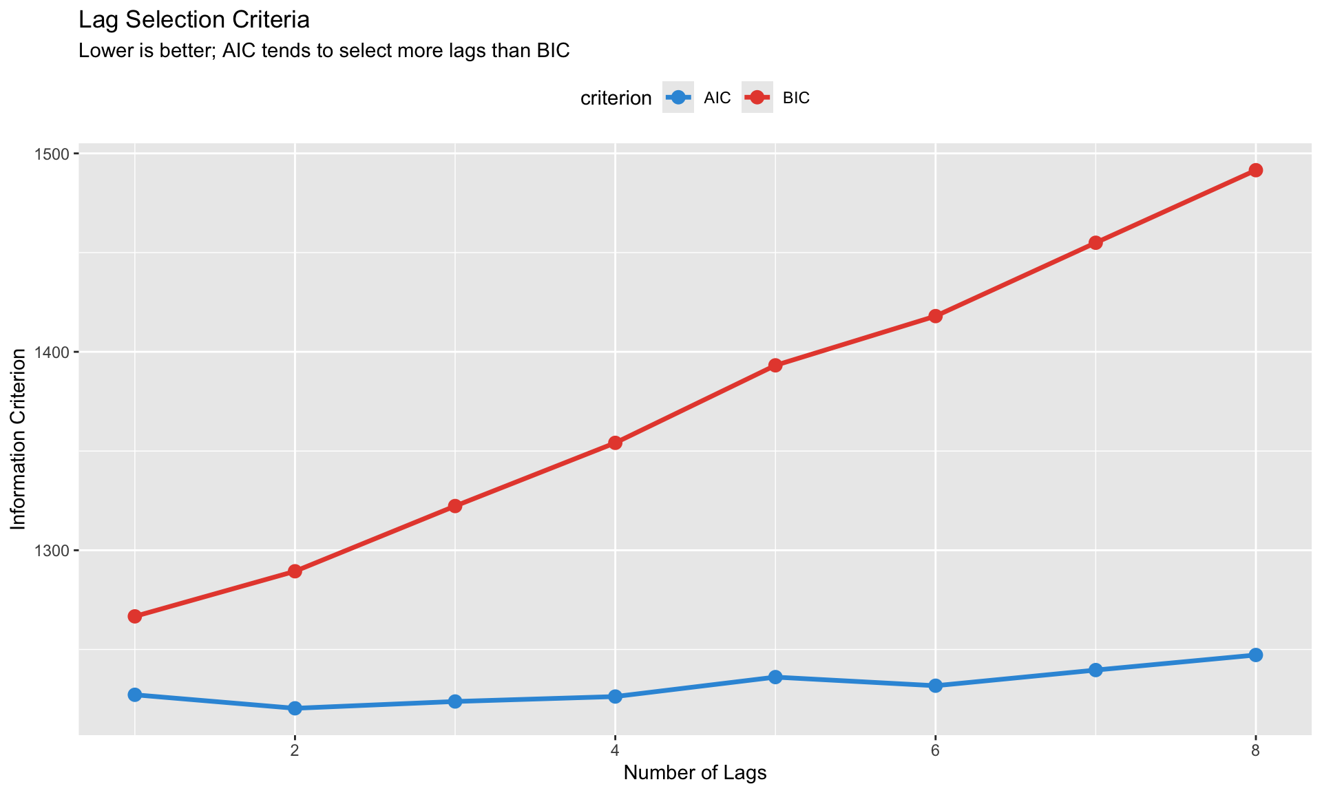
Model Selection and Diagnostics

Lag Length Selection

Residual Diagnostics

Portmanteau Test for Serial Correlation:

Test statistic: 72.25

p-value: 0.9148

Interpretation: No significant serial correlation (good)

Summary Checklist

Before trusting your VAR results:

Stability: All eigenvalues inside unit circle?
Lag length: Information criteria checked? Residual autocorrelation tests passed?
Identification: Assumptions documented? Robustness to alternatives checked?
Sample size: Enough observations relative to parameters?
Structural breaks: Any reason to believe relationships changed?

LP vs. VAR: When to Use Which

Equivalence Result

Theorem (Plagborg-Møller & Wolf, 2021): Under correct specification, LP and VAR estimate the same population IRFs.

Practical Differences

Aspect	VAR	LP
Specification	Full system	Horizon-by-horizon
Efficiency	More efficient if correct	Less efficient
Robustness	Sensitive to misspecification	Robust
Nonlinearity	Difficult (threshold VAR)	Easy (interactions)
Confidence intervals	Tighter	Wider (but honest)
Output	IRFs, FEVD, historical decomp	IRFs only

Recommendations

Use VAR when: - You want FEVD or historical decomposition - System is well-specified and identified - Short horizons with good theoretical grounding

Use LP when: - Single shock identification only - State-dependence or nonlinearity matters - Robustness to misspecification is priority - Panel data

Summary

Key takeaways from this module:

VARs model joint dynamics without imposing much structure—but this flexibility comes with an identification cost
The identification problem: Reduced-form tells us correlations; we need assumptions for causation
Cholesky identification is simple but ordering-sensitive—always check robustness
Sign restrictions are more robust but set-identified—report the range of admissible models
External instruments can achieve point identification with plausible exogeneity—report the F-statistic
FEVD and historical decomposition require structural identification—interpret with caution
LP and VAR are complements: Use LP for robustness, VAR for richer output

Next: Module 5: Staggered Difference-in-Differences