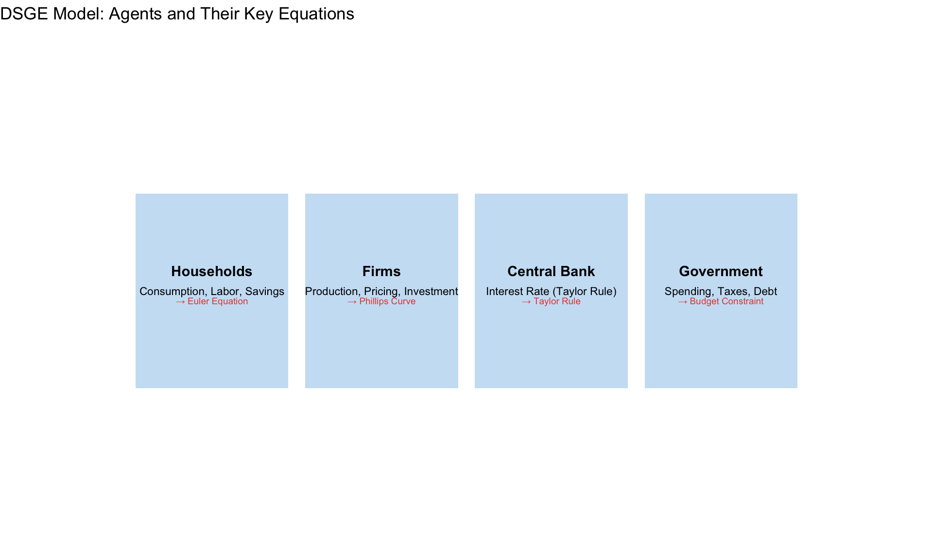
DSGE Foundations
Microfoundations, the New Keynesian Model, and Solution Methods
What is a DSGE Model?
Dynamic Stochastic General Equilibrium models are the workhorse of modern macroeconomics. They combine:
| Component | Meaning |
|---|---|
| Dynamic | Agents optimize over time, considering future |
| Stochastic | Random shocks drive business cycle fluctuations |
| General | All markets (goods, labor, capital) interact |
| Equilibrium | Supply equals demand in every market |
NoteThe Core Philosophy
DSGE models are microfounded: aggregate behavior emerges from explicit optimization by households, firms, and policymakers. No ad hoc aggregate relationships.
From Micro to Macro
The General Form
All DSGE models can be written as:
\[ \mathbb{E}_t\left[f(y_{t+1}, y_t, y_{t-1}, u_t)\right] = 0 \]
where:
- \(y_t\) = vector of endogenous variables (output, inflation, interest rate, capital, …)
- \(u_t\) = vector of exogenous shocks (technology, monetary, fiscal, …)
- \(f\) = system of equilibrium conditions (Euler equations, market clearing, …)
- \(\mathbb{E}_t\) = expectation conditional on time-\(t\) information
The challenge: solving for \(y_t\) as a function of states and shocks.
The RBC Core
Before New Keynesian elements, we start with the Real Business Cycle foundation.
Household Problem
A representative household maximizes expected lifetime utility:
\[ \max_{\{C_t, N_t, K_t\}} \mathbb{E}_0 \sum_{t=0}^{\infty} \beta^t U(C_t, N_t) \]
Subject to budget constraint: \[ C_t + K_t = W_t N_t + R_t^K K_{t-1} + \Pi_t - T_t + (1-\delta)K_{t-1} \]
where: - \(C_t\) = consumption - \(N_t\) = labor supply - \(K_t\) = end-of-period capital - \(W_t\) = real wage - \(R_t^K\) = rental rate on capital - \(\delta\) = depreciation rate - \(\Pi_t\) = firm profits - \(T_t\) = lump-sum taxes
First-Order Conditions
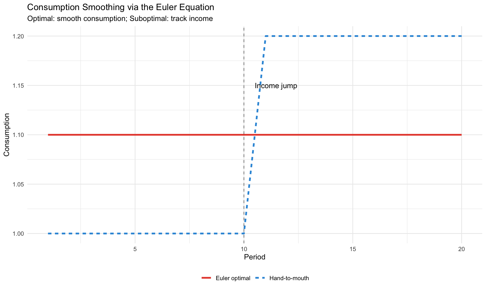
Euler equation (intertemporal consumption choice): \[ U_C(C_t, N_t) = \beta \mathbb{E}_t\left[U_C(C_{t+1}, N_{t+1}) \cdot (R_{t+1}^K + 1 - \delta)\right] \]
Labor supply (consumption-leisure trade-off): \[ \frac{-U_N(C_t, N_t)}{U_C(C_t, N_t)} = W_t \]
Example: Log Utility
With \(U(C, N) = \log(C) - \chi \frac{N^{1+\phi}}{1+\phi}\):
\[ \frac{1}{C_t} = \beta \mathbb{E}_t\left[\frac{1}{C_{t+1}} (R_{t+1}^K + 1 - \delta)\right] \]
\[ \chi N_t^\phi \cdot C_t = W_t \]
Firm Problem
A representative firm maximizes profits with Cobb-Douglas production:
\[ Y_t = A_t K_{t-1}^\alpha N_t^{1-\alpha} \]
Factor demands (competitive markets, firms are price-takers): \[ W_t = (1-\alpha) \frac{Y_t}{N_t} \] \[ R_t^K = \alpha \frac{Y_t}{K_{t-1}} \]
Technology shock follows AR(1): \[ \log(A_t) = \rho_A \log(A_{t-1}) + \varepsilon_{A,t}, \quad \varepsilon_{A,t} \sim N(0, \sigma_A^2) \]
Market Clearing
\[ Y_t = C_t + I_t \]
where investment \(I_t = K_t - (1-\delta)K_{t-1}\).
The Complete RBC Model
| Equation | Name | Variables |
|---|---|---|
| \(\frac{1}{C_t} = \beta \mathbb{E}_t\left[\frac{1}{C_{t+1}}(R_{t+1}^K + 1 - \delta)\right]\) | Euler | \(C, R^K\) |
| \(\chi N_t^\phi C_t = W_t\) | Labor supply | \(N, C, W\) |
| \(Y_t = A_t K_{t-1}^\alpha N_t^{1-\alpha}\) | Production | \(Y, A, K, N\) |
| \(W_t = (1-\alpha) Y_t / N_t\) | Labor demand | \(W, Y, N\) |
| \(R_t^K = \alpha Y_t / K_{t-1}\) | Capital demand | \(R^K, Y, K\) |
| \(Y_t = C_t + K_t - (1-\delta)K_{t-1}\) | Resource | \(Y, C, K\) |
| \(\log A_t = \rho_A \log A_{t-1} + \varepsilon_A\) | Technology | \(A\) |
7 equations, 7 unknowns: \((Y, C, N, K, W, R^K, A)\)
The New Keynesian Model
The RBC model has no role for monetary policy (all real). The New Keynesian model adds:
- Nominal rigidities (sticky prices/wages)
- Monopolistic competition (firms have pricing power)
- Monetary policy (central bank sets interest rate)
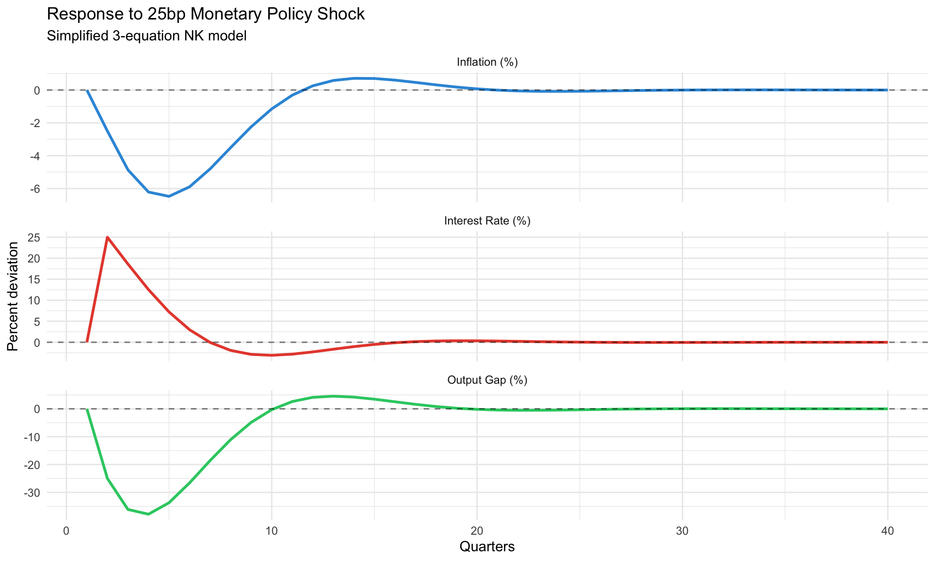
The 3-Equation NK Model
The canonical log-linearized NK model:
1. IS Curve (Dynamic IS)
From the household’s Euler equation: \[ \hat{y}_t = \mathbb{E}_t[\hat{y}_{t+1}] - \frac{1}{\sigma}(i_t - \mathbb{E}_t[\pi_{t+1}] - r_t^n) \]
where: - \(\hat{y}_t\) = output gap (deviation from flexible-price equilibrium) - \(i_t\) = nominal interest rate - \(\pi_t\) = inflation - \(r_t^n\) = natural rate of interest - \(\sigma\) = inverse elasticity of intertemporal substitution
Interpretation: Higher real interest rate → postpone consumption → lower output today.
2. Phillips Curve (NKPC)
From Calvo pricing (fraction \(1-\theta\) of firms adjust each period): \[ \pi_t = \beta \mathbb{E}_t[\pi_{t+1}] + \kappa \hat{y}_t \]
where: \[ \kappa = \frac{(1-\theta)(1-\beta\theta)}{\theta} \cdot (\sigma + \phi) \]
Interpretation: Inflation today depends on expected future inflation plus current output gap (marginal cost pressure).
3. Taylor Rule
Central bank sets interest rate: \[ i_t = \rho_i i_{t-1} + (1-\rho_i)\left[r^* + \phi_\pi(\pi_t - \pi^*) + \phi_y \hat{y}_t\right] + \varepsilon_{m,t} \]
Standard calibration:
| Parameter | Value | Interpretation |
|---|---|---|
| \(\rho_i\) | 0.8 | Interest rate smoothing |
| \(\phi_\pi\) | 1.5 | Response to inflation (Taylor principle: \(\phi_\pi > 1\)) |
| \(\phi_y\) | 0.5/4 = 0.125 | Response to output gap (quarterly) |
Deriving the Phillips Curve
Calvo Pricing Setup
- Each period, fraction \(1-\theta\) of firms can reset prices
- Fraction \(\theta\) are “stuck” with last period’s price
- When firms can adjust, they set price to maximize expected profits over the time they’ll be stuck
Optimal Price Setting
A firm that can adjust at time \(t\) chooses \(P_t^*\) to maximize: \[ \mathbb{E}_t \sum_{k=0}^{\infty} (\beta\theta)^k \left[ \frac{P_t^*}{P_{t+k}} Y_{t+k|t} - MC_{t+k} Y_{t+k|t} \right] \]
Result (after log-linearization): \[ \hat{p}_t^* = (1-\beta\theta) \sum_{k=0}^{\infty} (\beta\theta)^k \mathbb{E}_t[\widehat{mc}_{t+k}] \]
Firms set prices as a weighted average of expected future marginal costs.
Aggregating to the Phillips Curve
Price index evolution: \[ P_t = \left[\theta P_{t-1}^{1-\epsilon} + (1-\theta)(P_t^*)^{1-\epsilon}\right]^{\frac{1}{1-\epsilon}} \]
Log-linearizing and combining: \[ \pi_t = \beta \mathbb{E}_t[\pi_{t+1}] + \kappa \cdot \widehat{mc}_t \]
With \(\widehat{mc}_t \propto \hat{y}_t\) (output gap approximates marginal cost deviations).
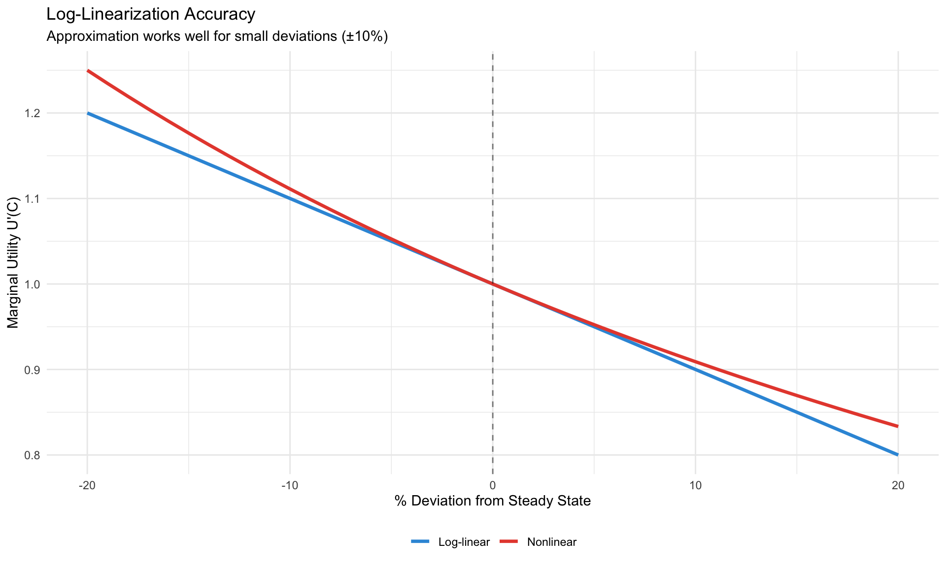
Log-Linearization
DSGE models are nonlinear. To solve them analytically (or with first-order perturbation), we log-linearize around the steady state.
The Technique
For any variable \(X_t\):
\[ \hat{x}_t \equiv \log(X_t) - \log(\bar{X}) = \log\left(\frac{X_t}{\bar{X}}\right) \approx \frac{X_t - \bar{X}}{\bar{X}} \]
So \(\hat{x}_t\) is the percentage deviation from steady state.
Key Approximation
For any function \(f(X_t, Y_t)\): \[ f(X_t, Y_t) \approx f(\bar{X}, \bar{Y}) + f_X(\bar{X}, \bar{Y})(X_t - \bar{X}) + f_Y(\bar{X}, \bar{Y})(Y_t - \bar{Y}) \]
Example: Euler Equation
Nonlinear Euler: \[ \frac{1}{C_t} = \beta \mathbb{E}_t\left[\frac{1}{C_{t+1}} R_{t+1}\right] \]
Step 1: Steady state \[ \frac{1}{\bar{C}} = \beta \frac{1}{\bar{C}} \bar{R} \implies \bar{R} = \frac{1}{\beta} \]
Step 2: Log-linearize. Let \(C_t = \bar{C} e^{\hat{c}_t} \approx \bar{C}(1 + \hat{c}_t)\): \[ \frac{1}{\bar{C}(1 + \hat{c}_t)} = \beta \mathbb{E}_t\left[\frac{1}{\bar{C}(1 + \hat{c}_{t+1})} \bar{R}(1 + \hat{r}_{t+1})\right] \]
Step 3: First-order Taylor expansion (ignore second-order terms): \[ 1 - \hat{c}_t = \beta \bar{R} \mathbb{E}_t\left[(1 - \hat{c}_{t+1})(1 + \hat{r}_{t+1})\right] \] \[ 1 - \hat{c}_t \approx \mathbb{E}_t[1 - \hat{c}_{t+1} + \hat{r}_{t+1}] \]
Result: \[ \hat{c}_t = \mathbb{E}_t[\hat{c}_{t+1}] - (\hat{r}_{t+1} - 0) \]
This is the log-linearized Euler equation (with \(\sigma = 1\)).
Solving Rational Expectations Models
After log-linearization, DSGE models take the form:
\[ A \mathbb{E}_t[y_{t+1}] = B y_t + C u_t \]
where \(y_t\) contains both predetermined (state) and jump (control) variables.
Partitioning the System
Split \(y_t = \begin{pmatrix} x_t \\ z_t \end{pmatrix}\) where:
- \(x_t\): Predetermined (state) variables — known at time \(t\) (e.g., capital \(K_{t-1}\))
- \(z_t\): Jump (forward-looking) variables — can adjust freely (e.g., consumption, inflation)
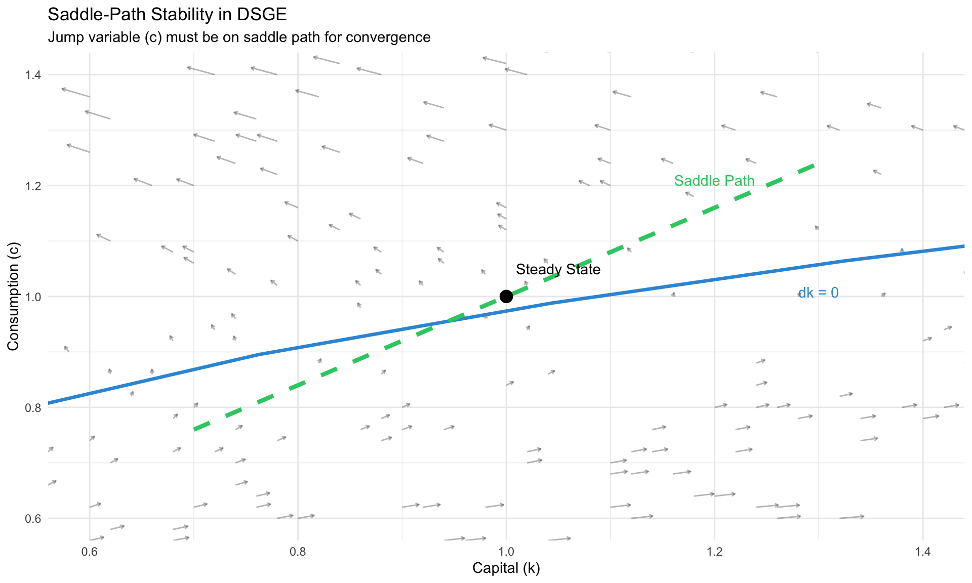
Blanchard-Kahn Conditions
The eigenvalue decomposition of the system matrix determines solvability (Blanchard and Kahn 1980).
ImportantBlanchard-Kahn (1980) Conditions
For a unique stable solution:
Number of eigenvalues outside unit circle = Number of jump variables
| Eigenvalue Count | Diagnosis |
|---|---|
| Equals number of jump vars | Unique solution (saddle-path stable) |
| Less than number of jump vars | Indeterminacy (multiple equilibria, sunspots) |
| Greater than number of jump vars | No solution (explosive dynamics) |
The Solution Form
If BK conditions hold, the solution is:
\[ x_{t+1} = H_x x_t + H_u u_{t+1} \] \[ z_t = G_x x_t \]
The policy function \(G_x\) tells us how jump variables respond to states. The transition matrix \(H_x\) governs state evolution.
Common Causes of BK Violations
| Problem | Symptom | Common Fix |
|---|---|---|
| Taylor principle violated | Too few unstable roots | Raise \(\phi_\pi\) above 1 |
| Missing expectations | Wrong root count | Check all \(\mathbb{E}_t\) terms |
| Timing error | Explosive solutions | Dynare uses end-of-period capital: use \(K(-1)\) |
| Wrong variable classification | Indeterminacy | Re-check predetermined vs. jump |
Numerical Solution: QZ Decomposition
For larger models, we use the generalized Schur (QZ) decomposition:
\[ A = Q \Lambda Z', \quad B = Q \Omega Z' \]
where \(\Lambda/\Omega\) gives generalized eigenvalues. Reorder to put unstable eigenvalues in the bottom block.
# R code sketch for BK solution
solve_dsge_bk <- function(A, B, n_state) {
  # A * E[y_{t+1}] = B * y_t
  # y = [x; z] where x = states, z = jumps

  n_total <- nrow(A)
  n_jump <- n_total - n_state

  # QZ decomposition
  qz <- geigen::gqz(A, B)  # Generalized Schur

  # Eigenvalues
  eig <- qz$alpha / qz$beta
  n_unstable <- sum(abs(eig) > 1)

  # Check BK conditions
  if (n_unstable != n_jump) {
    stop(paste("BK violation:", n_unstable, "unstable,", n_jump, "jump vars"))
  }

  # Extract policy function (from stable block)
  # ... (reorder and partition)

  list(G = G_matrix, H = H_matrix, eigenvalues = eig)
}
Calibration
Before estimation (Module 11), we calibrate parameters using:
- Microeconomic evidence (labor supply elasticity, depreciation rate)
- Long-run averages (capital-output ratio, hours worked)
- Steady-state relationships (Euler equation pins down \(\beta\))
Standard RBC/NK Calibration
| Parameter | Symbol | Value | Source |
|---|---|---|---|
| Discount factor | \(\beta\) | 0.99 | Real interest rate ≈ 4% annually |
| Capital share | \(\alpha\) | 0.33 | National accounts |
| Depreciation | \(\delta\) | 0.025 | 10% annual depreciation |
| Risk aversion | \(\sigma\) | 1-2 | Micro studies |
| Frisch elasticity | \(1/\phi\) | 0.5-2 | Labor supply literature |
| Calvo parameter | \(\theta\) | 0.75 | Prices adjust every 4 quarters |
| Inflation weight | \(\phi_\pi\) | 1.5 | Taylor (1993) |
| Output weight | \(\phi_y\) | 0.125 | Taylor (1993), quarterly |
Matching Moments
Target: Model-implied moments ≈ Data moments
| Moment | Data (US) | Typical RBC |
|---|---|---|
| std(Y) | 1.5-2% | Match by calibrating \(\sigma_A\) |
| std(C)/std(Y) | 0.5-0.7 | Endogenous |
| std(I)/std(Y) | 2.5-3.5 | Endogenous |
| corr(C, Y) | 0.8-0.9 | Endogenous |
| corr(N, Y) | 0.8-0.9 | Endogenous |
| Variable | Std Dev (%)_Model | Std Dev (%)_Data | Rel to Y_Model | Rel to Y_Data | Corr with Y_Model | Corr with Y_Data |
|---|---|---|---|---|---|---|
| Output | 2.26 | 1.8 | 1.00 | 1.00 | 1.00 | 1.00 |
| Consumption | 1.60 | 1.0 | 0.71 | 0.55 | 0.99 | 0.85 |
| Investment | 6.77 | 5.0 | 2.99 | 2.80 | 1.00 | 0.90 |
| Hours | 1.14 | 1.5 | 0.50 | 0.83 | 0.96 | 0.85 |
Calibration: matching business cycle moments
Steady-State Relationships
Many parameters are pinned down by steady-state conditions:
From Euler equation: \[ \bar{R} = \frac{1}{\beta} \implies \beta = \frac{1}{1 + r^*} \] With \(r^* = 4\%\) annually → \(\beta = 1/1.01 \approx 0.99\) quarterly.
From capital demand: \[ \bar{R}^K = \alpha \frac{\bar{Y}}{\bar{K}} = \frac{1}{\beta} - (1-\delta) \] Given \(\beta\), \(\delta\), and capital-output ratio, backs out \(\alpha\).
From labor supply: \[ \chi \bar{N}^\phi \bar{C} = \bar{W} = (1-\alpha)\frac{\bar{Y}}{\bar{N}} \] Given target \(\bar{N} = 1/3\) (8 hours/day), backs out \(\chi\).
Dynare Basics
Dynare is the standard software for solving and estimating DSGE models. Here’s a minimal example.
A Simple RBC Model in Dynare
%% RBC Model - rbc_simple.mod
%% Preamble
var y c k n w r a;
varexo eps_a;
parameters BETA ALPHA DELTA RHO_A SIGMA_A CHI PHI;

%% Calibration
BETA = 0.99;
ALPHA = 0.33;
DELTA = 0.025;
RHO_A = 0.95;
SIGMA_A = 0.007;
CHI = 1;       % labor disutility
PHI = 1;       % inverse Frisch elasticity

%% Model equations
model;
  % Euler equation
  1/c = BETA * (1/c(+1)) * (r(+1) + 1 - DELTA);

  % Labor supply
  CHI * n^PHI * c = w;

  % Production function
  y = a * k(-1)^ALPHA * n^(1-ALPHA);

  % Factor prices
  w = (1-ALPHA) * y / n;
  r = ALPHA * y / k(-1);

  % Resource constraint
  y = c + k - (1-DELTA)*k(-1);

  % Technology shock
  log(a) = RHO_A * log(a(-1)) + eps_a;
end;

%% Steady state
initval;
  a = 1;
  r = 1/BETA - 1 + DELTA;
  k = (ALPHA/r)^(1/(1-ALPHA)) * 0.33;
  n = 0.33;
  y = a * k^ALPHA * n^(1-ALPHA);
  c = y - DELTA*k;
  w = (1-ALPHA) * y / n;
end;

steady;
check;

%% Shocks
shocks;
  var eps_a; stderr SIGMA_A;
end;

%% Simulation
stoch_simul(order=1, irf=40, periods=200);
Key Dynare Commands
| Command | Purpose |
|---|---|
steady |
Compute deterministic steady state |
check |
Verify Blanchard-Kahn conditions |
stoch_simul(order=1) |
First-order perturbation solution |
stoch_simul(irf=40) |
Generate IRFs for 40 periods |
estimation(...) |
Bayesian estimation (Module 11) |
model_diagnostics |
Check model specification |
Important Timing Convention
WarningDynare Timing
Dynare uses end-of-period capital: - k without subscript = \(K_t\) (end of period \(t\)) - k(-1) = \(K_{t-1}\) (beginning of period \(t\) = end of \(t-1\))
So the production function uses k(-1):
y = a * k(-1)^ALPHA * n^(1-ALPHA);Summary
| Concept | Key Insight |
|---|---|
| DSGE structure | Microfounded optimization → aggregate equilibrium |
| Households | Euler equation governs intertemporal choice |
| Firms (NK) | Calvo pricing → forward-looking Phillips curve |
| Monetary policy | Taylor rule with \(\phi_\pi > 1\) for stability |
| Log-linearization | Approximate around steady state for solution |
| Blanchard-Kahn | Saddle-path stability requires correct eigenvalue count |
| Calibration | Match parameters to micro evidence and steady-state targets |
TipNext Steps
Module 11 covers DSGE estimation: - Bayesian methods with Metropolis-Hastings - The Kalman filter for likelihood evaluation - Model comparison via marginal likelihood - Dynare’s estimation command
Key References
Foundational
- Kydland & Prescott (1982) “Time to Build and Aggregate Fluctuations” Econometrica — RBC origins
- Blanchard & Kahn (1980) “The Solution of Linear Difference Models” Econometrica — BK conditions
- Galí (2015) Monetary Policy, Inflation, and the Business Cycle — NK textbook
Medium-Scale Models
- Smets & Wouters (2003, 2007) “An Estimated DSGE Model” — Benchmark estimated NK
- Christiano, Eichenbaum & Evans (2005) “Nominal Rigidities” JPE — CEE model
Solution Methods
- Uhlig (1999) “A Toolkit for Analysing Nonlinear Dynamic Stochastic Models” — Perturbation
- Sims (2002) “Solving Linear Rational Expectations Models” — QZ decomposition
Calibration
- Cooley & Prescott (1995) “Economic Growth and Business Cycles” — Calibration methodology
- Chari, Kehoe & McGrattan (2007) “Business Cycle Accounting” Econometrica — Wedges approach
Software
- Adjemian et al. “Dynare” — Standard DSGE solver
- Herbst & Schorfheide (2016) Bayesian Estimation of DSGE Models — Modern estimation