Causal Machine Learning
Heterogeneous Treatment Effects, Causal Forests, and Double ML
# Python setup (run in your Python environment)
import numpy as np
import pandas as pd
np.random.seed(42)
From Prediction to Causation
Machine learning excels at prediction: minimizing \(\mathbb{E}[(Y - \hat{f}(X))^2]\). But economists care about causation: what happens to \(Y\) if we intervene on \(X\)?
| Goal | Question | Method |
|---|---|---|
| Prediction | What is \(\hat{y}\) given \(x\)? | Random forest, neural net, boosting |
| Causation | What happens to \(y\) if we change \(x\)? | Experiments, IV, DiD, RDD |
NoteThe Causal ML Revolution
Recent methods—causal forests, double ML, meta-learners—combine ML’s flexibility for high-dimensional data with causal inference’s focus on identification (Athey and Imbens 2019). The key insight: use ML for nuisance parameters (propensity scores, outcome models) while preserving valid causal inference. Key methodological foundations include causal forests (Wager and Athey 2018) and double/debiased ML (Chernozhukov et al. 2018).
Key Papers
| Paper | Contribution |
|---|---|
| Athey & Imbens (2016) | Recursive partitioning for heterogeneous causal effects |
| Wager & Athey (2018) | Causal forests with valid asymptotic inference |
| Chernozhukov et al. (2018) | Double/Debiased ML for high-dimensional controls |
| Künzel et al. (2019) | Meta-learners (X-learner) for CATE |
| Athey & Wager (2021) | Policy learning with observational data |
The Potential Outcomes Framework
Setup
For each unit \(i\):
- Treatment: \(W_i \in \{0, 1\}\)
- Potential outcomes: \(Y_i(0), Y_i(1)\) — what would happen under control/treatment
- Observed outcome: \(Y_i = W_i \cdot Y_i(1) + (1 - W_i) \cdot Y_i(0)\)
- Covariates: \(X_i\) (pre-treatment characteristics)
Treatment Effects Taxonomy
| Estimand | Definition | Interpretation |
|---|---|---|
| ITE | \(\tau_i = Y_i(1) - Y_i(0)\) | Individual effect (unobservable) |
| CATE | \(\tau(x) = \mathbb{E}[Y(1) - Y(0) \mid X = x]\) | Conditional average effect |
| ATE | \(\mathbb{E}[\tau_i]\) | Average treatment effect |
| ATT | \(\mathbb{E}[\tau_i \mid W_i = 1]\) | Effect on the treated |
The Fundamental Problem of Causal Inference
We observe either \(Y_i(1)\) OR \(Y_i(0)\), never both. The individual treatment effect \(\tau_i\) is fundamentally unidentifiable.
Solution: Under unconfoundedness (selection on observables): \[ (Y_i(0), Y_i(1)) \perp\!\!\!\perp W_i \mid X_i \]
Plus overlap (positivity): \(0 < P(W_i = 1 \mid X_i = x) < 1\) for all \(x\).
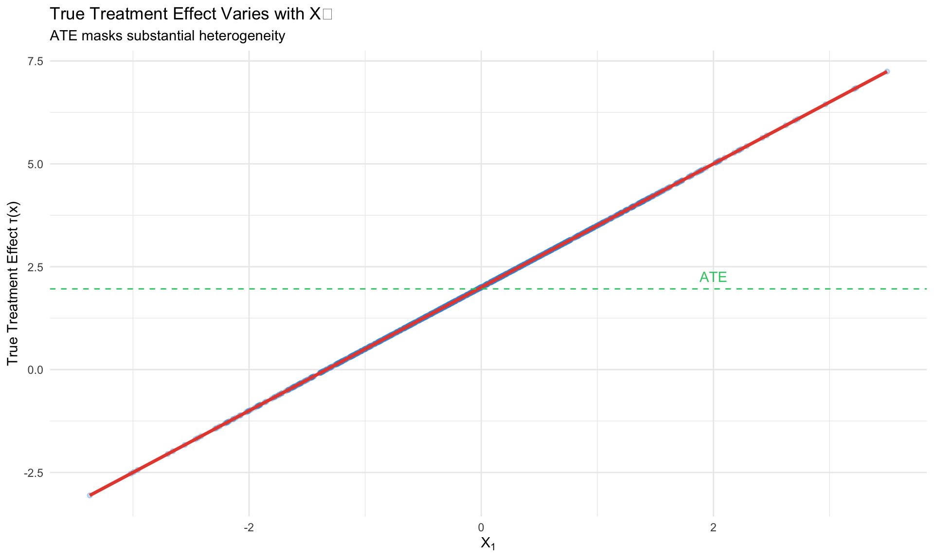
Heterogeneous Treatment Effects
Why Heterogeneity Matters
The ATE \(= 2\) could mask:
- Subgroup A: \(\tau = 5\) (strong benefit)
- Subgroup B: \(\tau = -1\) (harm)
Understanding heterogeneity enables:
- Targeting: Treat those who benefit most
- Mechanism identification: What drives variation?
- Policy optimization: Maximize welfare under constraints
Traditional Approaches and Their Limitations
Subgroup analysis: Pre-specify groups, estimate effects within each.
- Problem: Many possible subgroups → multiple testing
- Problem: Boundaries are arbitrary
Interaction terms: \(Y = \alpha + \tau W + \gamma W \cdot X + \beta X + \varepsilon\)
- Problem: Must specify functional form
- Problem: Doesn’t scale to many \(X\)
Causal ML: Learn \(\tau(x)\) flexibly from data with valid inference.
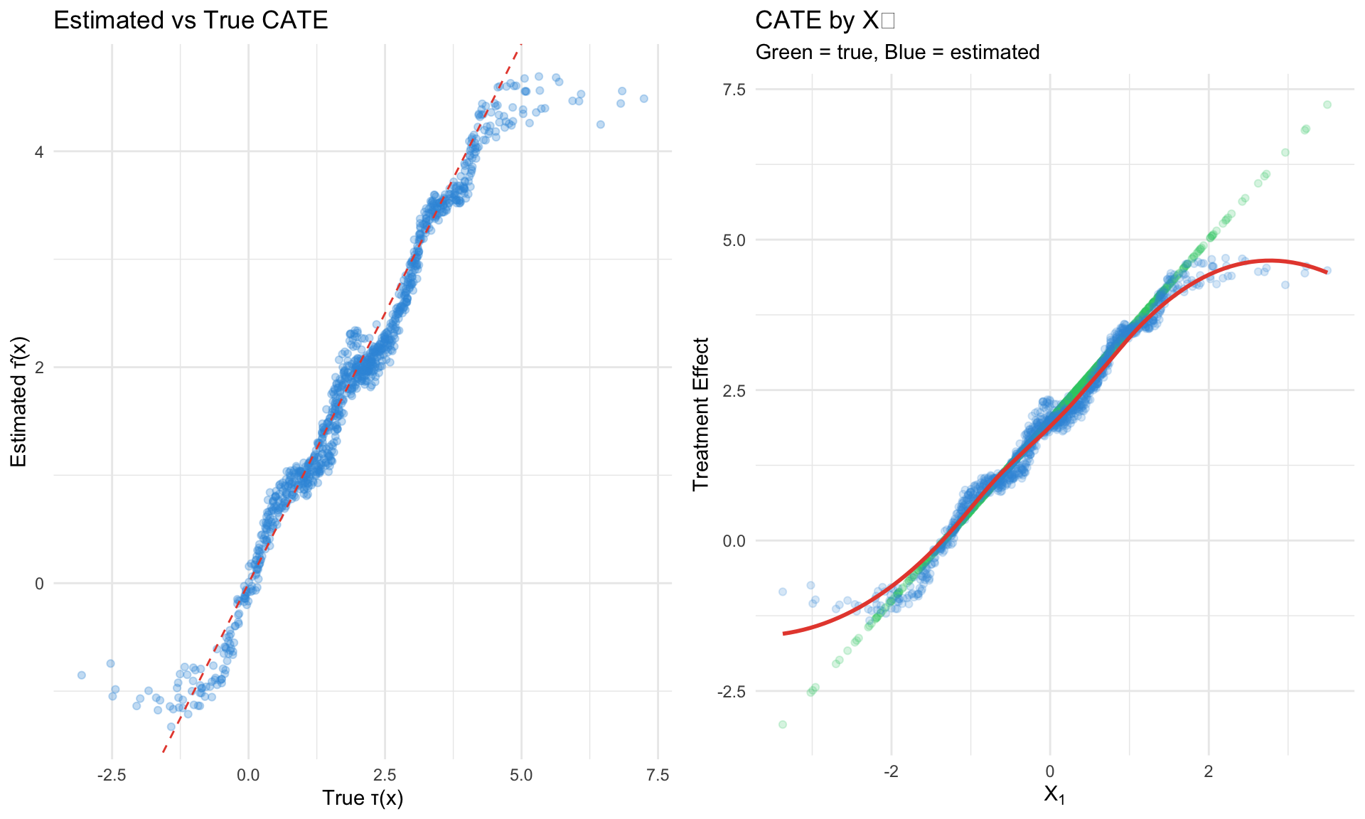
Causal Forests
The Key Idea (Wager & Athey 2018)
Adapt random forests from predicting \(\mathbb{E}[Y|X]\) to predicting \(\tau(x) = \mathbb{E}[Y(1) - Y(0)|X=x]\).
Key innovations:
- Honest splitting: Separate samples for tree structure vs. leaf estimation
- Heterogeneity-maximizing splits: Split to maximize treatment effect variation
- Valid inference: Asymptotic normality of estimates
Algorithm
For each tree \(b = 1, \ldots, B\):
- Subsample data into tree-building (\(\mathcal{I}_1\)) and estimation (\(\mathcal{I}_2\)) sets
- Build tree on \(\mathcal{I}_1\): at each node, find split maximizing heterogeneity
- Estimate leaf effects using \(\mathcal{I}_2\) only (honesty)
- Aggregate: \(\hat{\tau}(x) = \frac{1}{B} \sum_b \hat{\tau}_b(x)\)
R Implementation with grf
Key grf Functions
library(grf)
# Fit causal forest
cf <- causal_forest(X, Y, W, num.trees = 2000)
# Point predictions
tau_hat <- predict(cf)$predictions
# Predictions with variance (for CIs)
tau_ci <- predict(cf, estimate.variance = TRUE)
lower <- tau_ci$predictions - 1.96 * sqrt(tau_ci$variance.estimates)
upper <- tau_ci$predictions + 1.96 * sqrt(tau_ci$variance.estimates)
# Average treatment effect with SE
ate <- average_treatment_effect(cf, target.sample = "all")
cat("ATE:", ate[1], "SE:", ate[2], "\n")
# ATT
att <- average_treatment_effect(cf, target.sample = "treated")
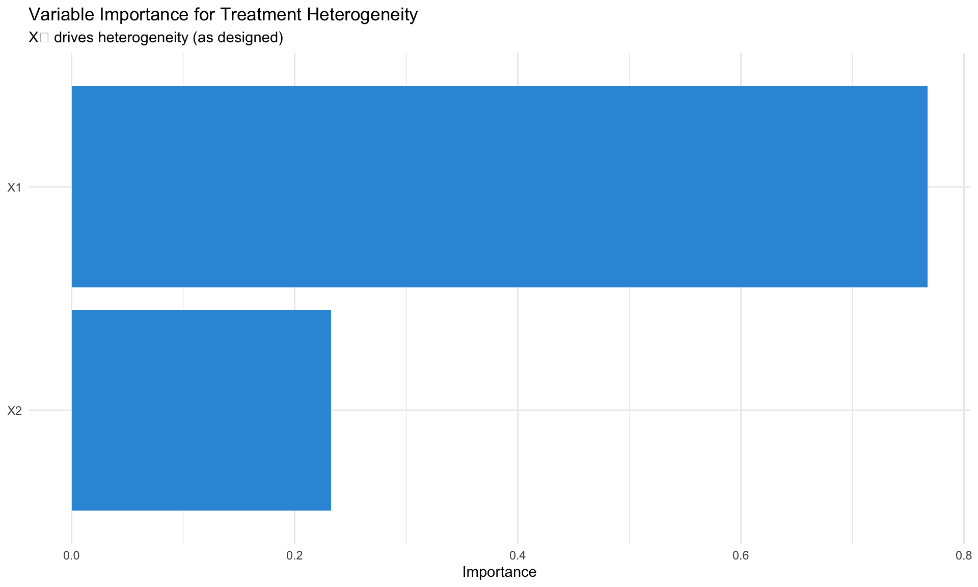
# Variable importance: which X drive heterogeneity?
vi <- variable_importance(cf)
# Best linear projection: linear approximation of τ(x)
blp <- best_linear_projection(cf, X)
# Calibration test: is there heterogeneity?
test_calibration(cf)Variable Importance
Which covariates drive treatment effect heterogeneity?
Observational Data: Pre-Estimated Nuisance Functions
For observational studies, pre-fit propensity and outcome models:
# Pre-fit nuisance models (recommended for observational data)
W.hat <- predict(regression_forest(X, W))$predictions  # propensity
Y.hat <- predict(regression_forest(X, Y))$predictions  # outcome

# Causal forest with pre-estimated nuisance
cf_obs <- causal_forest(X, Y, W, W.hat = W.hat, Y.hat = Y.hat)
Double/Debiased Machine Learning
The Problem
When using ML for nuisance parameters (propensity score, outcome model), regularization introduces bias that invalidates standard inference.
Example: LASSO shrinks coefficients → biased treatment effect → invalid t-statistics.
The Solution (Chernozhukov et al. 2018)
Two key ingredients:
- Cross-fitting: Train ML on fold \(-k\), predict on fold \(k\)
- Neyman orthogonality: Use score function robust to nuisance estimation error
Partially Linear Model
\[ Y = \theta D + g(X) + U, \quad \mathbb{E}[U|X,D] = 0 \] \[ D = m(X) + V, \quad \mathbb{E}[V|X] = 0 \]
Target: \(\theta\) (treatment effect)
Nuisance: \(g(X)\) (outcome confounding), \(m(X)\) (propensity/treatment model)
The Algorithm
- Split data into \(K\) folds (typically \(K = 5\))
- For each fold \(k\):
- Train \(\hat{g}_{-k}(X)\) and \(\hat{m}_{-k}(X)\) on all other folds
- Compute residuals on fold \(k\):
- \(\tilde{Y}_i = Y_i - \hat{g}_{-k}(X_i)\)
- \(\tilde{D}_i = D_i - \hat{m}_{-k}(X_i)\)
- Estimate: \(\hat{\theta} = \frac{\sum_i \tilde{D}_i \tilde{Y}_i}{\sum_i \tilde{D}_i^2}\)
- Standard error: standard OLS formula on residualized data
Why It Works: Orthogonality
The orthogonal moment condition: \[ \psi(W; \theta, \eta) = (Y - g(X) - \theta D)(D - m(X)) \]
has the property that small errors in \(\hat{g}, \hat{m}\) don’t bias \(\hat{\theta}\): \[ \frac{\partial}{\partial \eta} \mathbb{E}[\psi(W; \theta_0, \eta)] \bigg|_{\eta = \eta_0} = 0 \]
Python Implementation with doubleml
# Double ML estimation in Python
from sklearn.ensemble import RandomForestRegressor
from sklearn.model_selection import cross_val_predict
import warnings
warnings.filterwarnings('ignore')

# Simulate data
n = 2000
p = 10
X = np.random.randn(n, p)
theta_true = 0.5  # true treatment effect
D = X[:, 0] + 0.5 * X[:, 1] + np.random.randn(n)  # treatment depends on X
Y = theta_true * D + X[:, 0] + X[:, 1] + np.random.randn(n)  # outcome

# Manual Double ML
def double_ml_plr(Y, D, X, K=5):
    """
    Double ML for Partially Linear Regression
    Y = theta * D + g(X) + U
    D = m(X) + V
    """
    n = len(Y)

    # Cross-fitted predictions
    g_hat = cross_val_predict(
        RandomForestRegressor(n_estimators=100, max_depth=5, random_state=42),
        X, Y, cv=K
    )
    m_hat = cross_val_predict(
        RandomForestRegressor(n_estimators=100, max_depth=5, random_state=42),
        X, D, cv=K
    )

    # Residualize
    Y_tilde = Y - g_hat
    D_tilde = D - m_hat

    # Estimate theta
    theta_hat = np.sum(D_tilde * Y_tilde) / np.sum(D_tilde ** 2)

    # Standard error
    residuals = Y_tilde - theta_hat * D_tilde
    se_hat = np.sqrt(np.sum(residuals ** 2 * D_tilde ** 2) / (np.sum(D_tilde ** 2) ** 2))

    return {
        'estimate': theta_hat,
        'se': se_hat,
        'ci_lower': theta_hat - 1.96 * se_hat,
        'ci_upper': theta_hat + 1.96 * se_hat
    }

# Run Double ML
result = double_ml_plr(Y, D, X)

print(f"True θ: {theta_true}")
print(f"Double ML estimate: {result['estimate']:.4f}")
print(f"Standard error: {result['se']:.4f}")
print(f"95% CI: [{result['ci_lower']:.4f}, {result['ci_upper']:.4f}]")
Using the DoubleML Package
from doubleml import DoubleMLPLR, DoubleMLData
from sklearn.ensemble import RandomForestRegressor

# Create data object
df = pd.DataFrame(X, columns=[f'X{i}' for i in range(p)])
df['Y'] = Y
df['D'] = D

dml_data = DoubleMLData(
    df, y_col='Y', d_cols='D',
    x_cols=[f'X{i}' for i in range(p)]
)

# Specify learners
ml_l = RandomForestRegressor(n_estimators=500, max_depth=5)
ml_m = RandomForestRegressor(n_estimators=500, max_depth=5)

# Fit
dml_plr = DoubleMLPLR(dml_data, ml_l, ml_m, n_folds=5)
dml_plr.fit()
print(dml_plr.summary)
R Implementation
Double ML ATE: 1.864 SE: 0.084 True ATE: 1.961 95% CI: [ 1.699 , 2.029 ]Meta-Learners
Overview
Meta-learners are strategies for combining base ML models to estimate CATE.
T-Learner (Two Models)
Train separate models for treatment and control:
\[ \hat{\tau}(x) = \hat{\mu}_1(x) - \hat{\mu}_0(x) \]
# T-Learner implementation
from sklearn.ensemble import RandomForestRegressor

# Binary treatment simulation
n = 1000
X_sim = np.random.randn(n, 5)
W_sim = np.random.binomial(1, 0.5, n)
tau_sim = X_sim[:, 0] + 0.5 * X_sim[:, 1]
Y_sim = tau_sim * W_sim + X_sim[:, 0] + np.random.randn(n)

# T-Learner: separate models for treatment and control
model_0 = RandomForestRegressor(n_estimators=100, random_state=42)
model_1 = RandomForestRegressor(n_estimators=100, random_state=42)

model_0.fit(X_sim[W_sim == 0], Y_sim[W_sim == 0])
model_1.fit(X_sim[W_sim == 1], Y_sim[W_sim == 1])

tau_t = model_1.predict(X_sim) - model_0.predict(X_sim)

print(f"T-Learner correlation with true τ: {np.corrcoef(tau_sim, tau_t)[0,1]:.3f}")Pros: Simple, no propensity needed
Cons: High variance, especially with imbalanced treatment
S-Learner (Single Model)
Single model with treatment as feature:
\[ \hat{\mu}(x, w) \rightarrow \hat{\tau}(x) = \hat{\mu}(x, 1) - \hat{\mu}(x, 0) \]
# S-Learner: single model with treatment as feature
X_aug = np.column_stack([X_sim, W_sim])
model_s = RandomForestRegressor(n_estimators=100, random_state=42)
model_s.fit(X_aug, Y_sim)

# Predict under treatment and control
tau_s = (model_s.predict(np.column_stack([X_sim, np.ones(n)])) -
         model_s.predict(np.column_stack([X_sim, np.zeros(n)])))

print(f"S-Learner correlation with true τ: {np.corrcoef(tau_sim, tau_s)[0,1]:.3f}")Pros: Simple, regularization shared
Cons: Treatment effect can be shrunk to zero
X-Learner (Künzel et al. 2019)
Best for imbalanced treatment (few treated or few controls):
- Fit \(\hat{\mu}_0, \hat{\mu}_1\) (T-learner)
- Impute treatment effects:
- Treated: \(\tilde{D}_1 = Y_1 - \hat{\mu}_0(X_1)\)
- Control: \(\tilde{D}_0 = \hat{\mu}_1(X_0) - Y_0\)
- Fit models: \(\hat{\tau}_0(x), \hat{\tau}_1(x)\)
- Combine: \(\hat{\tau}(x) = e(x) \hat{\tau}_0(x) + (1-e(x)) \hat{\tau}_1(x)\)
Comparison
| Learner | Best When | Weakness |
|---|---|---|
| T-Learner | Balanced, large samples | High variance |
| S-Learner | Small effects, regularization needed | Shrinks effects |
| X-Learner | Imbalanced treatment | Complex, needs propensity |
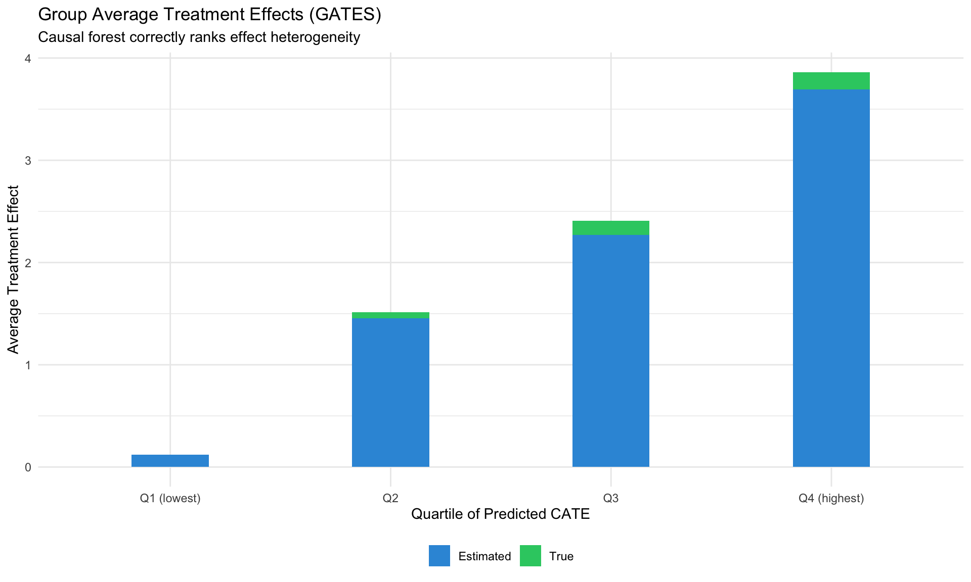
Group Average Treatment Effects (GATES)
Evaluating Heterogeneity
GATES groups units by predicted CATE and estimates average effects within each group:
Best Linear Predictor (BLP)
Which covariates explain heterogeneity?
Best linear projection of the conditional average treatment effect.
Confidence intervals are cluster- and heteroskedasticity-robust (HC3):

             Estimate Std. Error t value Pr(>|t|)
(Intercept)  1.923589   0.067767 28.3853   <2e-16 ***
X1           1.522921   0.074177 20.5308   <2e-16 ***
X2          -0.038501   0.071713 -0.5369   0.5915
---
Signif. codes:  0 '***' 0.001 '**' 0.01 '*' 0.05 '.' 0.1 ' ' 1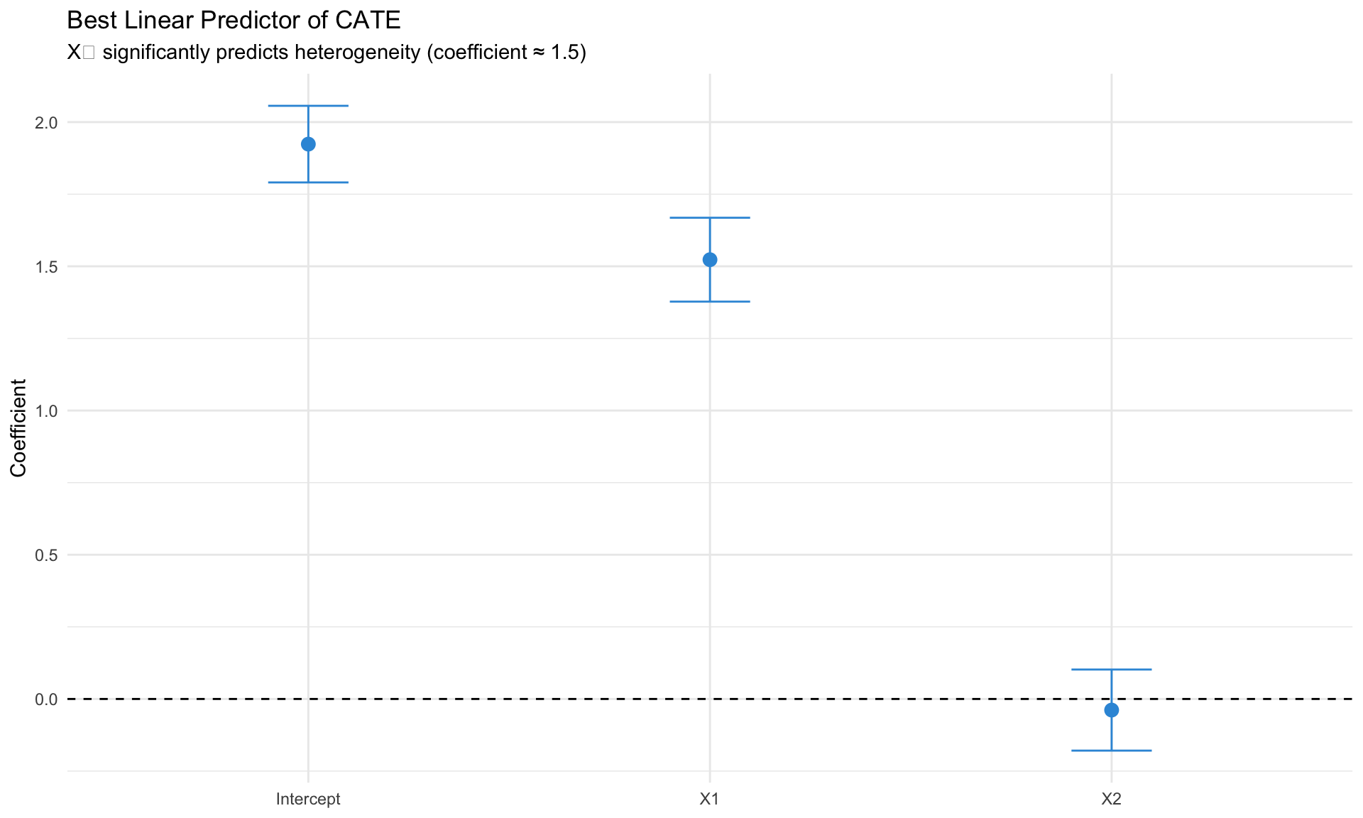
EconML: Microsoft’s Causal ML Toolkit
Overview
EconML provides a unified API for heterogeneous treatment effect estimation in Python.
Key Estimators
| Estimator | Description |
|---|---|
LinearDML |
DML with linear final stage |
CausalForestDML |
Causal forest with DML |
ForestDRLearner |
Doubly robust forest |
OrthoIV |
Orthogonal IV learner |
DynamicDML |
Panel data |
Python Implementation
# EconML example
from econml.dml import LinearDML, CausalForestDML
from sklearn.ensemble import RandomForestRegressor, RandomForestClassifier

# Setup
X_hetero = X_sim[:, :3]  # features for heterogeneity
W_confound = X_sim[:, 3:]  # confounders

# LinearDML
est_linear = LinearDML(
    model_y=RandomForestRegressor(n_estimators=100),
    model_t=RandomForestClassifier(n_estimators=100),
    cv=5
)
est_linear.fit(Y_sim, W_sim, X=X_hetero, W=W_confound)

# Effects
tau_linear = est_linear.effect(X_hetero)

# Inference
tau_lower, tau_upper = est_linear.effect_interval(X_hetero, alpha=0.05)

# Summary
print(est_linear.summary())
Unified API Pattern
All EconML estimators follow:
est.fit(Y, T, X=X, W=W)           # fit (Y=outcome, T=treatment, X=hetero, W=confound)
est.effect(X_test)                 # point estimates
est.effect_interval(X_test)        # confidence intervals
est.summary()                      # inference summary
Applications in Macroeconomics
Heterogeneous Policy Effects
Question: How do monetary policy effects vary across firms/regions/time?
Approach:
- Identify policy shocks (high-frequency, narrative)
- Estimate heterogeneous effects using causal forests
- Characterize which observables predict sensitivity
Example: Cross-Country Monetary Transmission
# Do bank holdings predict constrained monetary response?
cf_policy <- causal_forest(
  X = cbind(bank_holdings, cbi_index, debt_gdp, trade_openness),
  Y = delta_inflation,
  W = tightening_dummy
)

# Which characteristics drive heterogeneity?
variable_importance(cf_policy)

# Linear approximation
best_linear_projection(cf_policy,
                       cbind(bank_holdings, cbi_index, debt_gdp))
Fiscal Multiplier Heterogeneity
Do fiscal multipliers vary by:
- Slack (output gap)?
- Monetary policy stance (ZLB)?
- Debt levels?
Causal forests can flexibly estimate: \[ \text{Multiplier}(x) = \mathbb{E}[\Delta Y \mid \text{Fiscal shock}, X = x] \]
Practical Considerations
Sample Size Requirements
| Method | Minimum N | Recommended N |
|---|---|---|
| ATE (Double ML) | 200 | 500+ |
| CATE (Causal Forest) | 500 | 2000+ |
| GATES | 1000 | 3000+ |
| Variable Importance | 2000 | 5000+ |
Diagnostics
Overlap Check
# Propensity score distribution
e_hat <- cf$W.hat
hist(e_hat, breaks = 50, main = "Propensity Scores")
abline(v = c(0.1, 0.9), col = "red", lty = 2)

# Extreme values
cat("Extreme propensity:", mean(e_hat < 0.1 | e_hat > 0.9) * 100, "%\n")
Calibration Test
# Is there actually heterogeneity?
test_calibration(cf)
# Look for significant "differential.forest.prediction"
AUTOC (Targeting Quality)
# Area Under the TOC Curve
rate <- rank_average_treatment_effect(cf, X[, 1])
print(rate)  # CI should exclude 0
Common Pitfalls
- Causal ML doesn’t solve identification: Still need unconfoundedness
- Overfitting CATE: Use honest forests, cross-validation
- Noise as heterogeneity: Run calibration tests
- Overlap violations: Check propensity scores, trim extremes
- Small samples: CATE unreliable with N < 500
Summary
| Method | Purpose | Package |
|---|---|---|
| Causal Forest | Heterogeneous treatment effects | grf (R) |
| Double ML | ATE with high-dimensional controls | DoubleML (Python/R) |
| EconML | Unified CATE estimation | econml (Python) |
| Meta-Learners | T/S/X strategies for CATE | Various |
TipFor Macro Applications
- Sample sizes matter: Cross-country panels may be too small for CATE
- Identification first: Causal ML requires the same assumptions as traditional methods
- Focus on BLP and GATES: Which characteristics predict heterogeneity?
- Aggregation concerns: Individual effects may aggregate differently at macro level
Key References
Foundational
- Athey & Imbens (2016) “Recursive Partitioning for Heterogeneous Causal Effects” PNAS
- Wager & Athey (2018) “Estimation and Inference of Heterogeneous Treatment Effects using Random Forests” JASA
- Chernozhukov et al. (2018) “Double/Debiased Machine Learning” Econometrics Journal
Extensions
- Künzel et al. (2019) “Metalearners for Heterogeneous Treatment Effects” PNAS
- Athey & Wager (2021) “Policy Learning with Observational Data” Econometrica
- Kennedy (2022) “Optimal Doubly Robust Estimation of Heterogeneous Causal Effects”
Resources
- Causal ML Book: https://causalml-book.org/
- ML for Economists: https://github.com/ml4econ/lecture-notes-2025
- grf Documentation: https://grf-labs.github.io/grf/
- EconML: https://github.com/py-why/EconML
- DoubleML: https://github.com/DoubleML/doubleml-for-py