The Fundamental Problem
This section develops the core challenge of causal inference in macroeconomic settings: moving from observed correlations to credible causal estimates.
Why Correlation ≠ Causation
The Ideal Experiment
To measure the causal effect of a policy \(D\) on an outcome \(Y\), we would ideally observe:
\[
\tau_i = Y_i(1) - Y_i(0)
\]
where \(Y_i(1)\) is the outcome if unit \(i\) receives treatment, and \(Y_i(0)\) is the outcome if it doesn’t. The fundamental problem of causal inference is that we only observe one of these potential outcomes for each unit.
In macro settings, this is particularly severe: - We can’t randomly assign monetary policy across countries - We can’t rerun history with different fiscal rules - Countries that adopt different policies differ in many other ways
Three Sources of Bias
When we estimate \(\hat{\beta}\) from a regression of \(Y\) on \(X\), the estimate can be biased for the true causal effect \(\beta\) due to:
1. Simultaneity (Reverse Causality)
\[
X \rightarrow Y \quad \text{AND} \quad Y \rightarrow X
\]
Example: Do high interest rates cause low inflation, or does low inflation allow central banks to keep rates high? The regression coefficient captures both directions.
2. Selection (Confounding)
\[
Z \rightarrow X \quad \text{AND} \quad Z \rightarrow Y
\]
Example: Countries with strong institutions (\(Z\)) both adopt prudent debt management (\(X\)) and have stable monetary policy (\(Y\)). The correlation between \(X\) and \(Y\) reflects their common cause \(Z\).
3. Omitted Variables
A special case of confounding where the confounder \(Z\) is unobserved:
\[
\hat{\beta}_{OLS} \xrightarrow{p} \beta + \underbrace{\gamma \cdot \frac{\text{Cov}(X, Z)}{\text{Var}(X)}}_{\text{omitted variable bias}}
\]
where \(\gamma\) is the effect of \(Z\) on \(Y\).
Why “Controlling For” Doesn’t Solve It
A common but flawed intuition: “Just add more controls to the regression.”
Problem 1: Bad Controls
Adding post-treatment variables can introduce bias. If \(M\) is affected by treatment:
D → M → Y (M is a mediator)
Controlling for \(M\) blocks part of the causal effect of \(D\) on \(Y\).
Problem 2: Unobservables
You can only control for what you observe. In macro: - Institutional quality is hard to measure - Political constraints are unobserved - Market expectations are latent
Problem 3: Measurement Error
Controls measured with error don’t fully absorb confounding:
\[
\tilde{Z} = Z + \nu \quad \Rightarrow \quad \text{bias persists even after controlling for } \tilde{Z}
\]
Modern applied economics requires more than “throwing in controls.” It requires an identification strategy—a credible argument for why the remaining variation in \(X\) is as good as randomly assigned conditional on the research design.
Directed Acyclic Graphs (DAGs)
DAGs provide a visual language for identification arguments.
Confounding structure:
    Z
   / \
  ↓   ↓
  X → Y
In this DAG, \(Z\) is a confounder: it causes both \(X\) and \(Y\). The path \(X \leftarrow Z \rightarrow Y\) creates a spurious correlation between \(X\) and \(Y\) even if \(X\) has no causal effect on \(Y\).
Key DAG concepts:
| Confounder |
Common cause of \(X\) and \(Y\) |
Must control for it (or use design) |
| Mediator |
On causal path from \(X\) to \(Y\) |
Don’t control for it |
| Collider |
Caused by both \(X\) and \(Y\) |
Don’t control for it |
| Backdoor path |
Non-causal path from \(X\) to \(Y\) |
Must block to identify causal effect |
Fixed Effects as Partial Solution
Panel fixed effects address one specific source of bias: time-invariant confounders.
\[
Y_{it} = \alpha_i + X_{it}'\beta + \varepsilon_{it}
\]
The country fixed effect \(\alpha_i\) absorbs all factors that: - Differ across countries - Don’t change over time
This includes: geography, colonial history, legal origin, language, etc.
What FE doesn’t solve: - Time-varying confounders - Reverse causality - Selection into treatment timing
From weakest to strongest causal claims:
- Cross-sectional correlation: Countries with high \(X\) have high \(Y\)
- Panel FE: When a country’s \(X\) rises, its \(Y\) rises (within-country)
- DiD: Countries exposed to shock saw \(Y\) change relative to unexposed (parallel trends)
- IV: Exogenous variation in \(X\) (from instrument) causes \(Y\) to change
- RCT: Random assignment of \(X\) (rare in macro)
Difference-in-Differences
DiD exploits variation from discrete policy changes or shocks to identify causal effects.
The Classic 2×2 Design
Consider a policy implemented in some countries (“treated”) at time \(T_0\), with other countries as controls.
Setup: - \(D_i = 1\) if country \(i\) is treated, 0 otherwise - \(Post_t = 1\) if \(t > T_0\), 0 otherwise
Regression: \[
Y_{it} = \alpha + \beta_1 D_i + \beta_2 Post_t + \tau (D_i \times Post_t) + \varepsilon_{it}
\]
The DiD estimator: \[
\hat{\tau}_{DiD} = \underbrace{(\bar{Y}_{T,Post} - \bar{Y}_{T,Pre})}_{\text{Treated change}} - \underbrace{(\bar{Y}_{C,Post} - \bar{Y}_{C,Pre})}_{\text{Control change}}
\]
This “differences out” both: - Permanent differences between treated and control (first difference) - Common time trends (second difference)
# Simulate DiD data
N <- 100
T_periods <- 10
T0 <- 5 # Treatment at period 5
did_data <- expand.grid(
unit = 1:N,
time = 1:T_periods
) %>%
mutate(
treated = unit <= N/2, # First half treated
post = time > T0,
# Parallel trends in potential outcomes
Y0 = 2 + 0.3 * time + ifelse(treated, 1, 0) + rnorm(n(), 0, 0.5),
# Treatment effect of 2 units
Y1 = Y0 + 2,
# Observed outcome
Y = ifelse(treated & post, Y1, Y0)
)
# Plot
did_summary <- did_data %>%
group_by(treated, time) %>%
summarise(Y = mean(Y), .groups = "drop")
ggplot(did_summary, aes(x = time, y = Y, color = treated, linetype = treated)) +
geom_line(size = 1.2) +
geom_vline(xintercept = T0, linetype = "dashed", alpha = 0.5) +
geom_segment(aes(x = T0, xend = T_periods,
y = 2 + 0.3*T0 + 1 + 0.3*(T_periods - T0),
yend = 2 + 0.3*T_periods + 1),
color = "gray50", linetype = "dotted", size = 0.8) +
annotate("text", x = T0 + 0.5, y = 3, label = "Treatment", hjust = 0) +
annotate("text", x = T_periods - 1, y = 5.8, label = "Counterfactual", color = "gray50") +
scale_color_manual(values = c("FALSE" = "#3498db", "TRUE" = "#e74c3c"),
labels = c("Control", "Treated")) +
scale_linetype_manual(values = c("FALSE" = "solid", "TRUE" = "solid"),
labels = c("Control", "Treated")) +
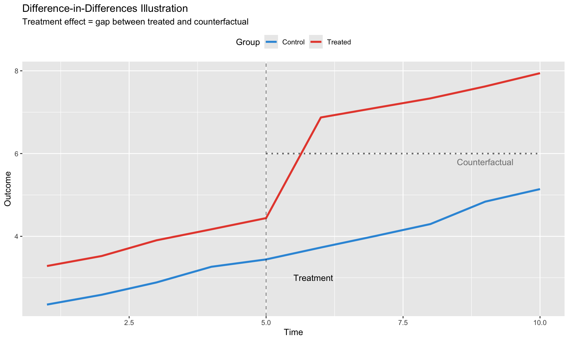
labs(title = "Difference-in-Differences Illustration",
subtitle = "Treatment effect = gap between treated and counterfactual",
x = "Time", y = "Outcome", color = "Group", linetype = "Group") +
theme(legend.position = "top")
The Parallel Trends Assumption
Assumption: In the absence of treatment, treated and control groups would have followed parallel paths.
\[
E[Y_{it}(0) | D_i = 1, t] - E[Y_{it}(0) | D_i = 0, t] = \delta \quad \forall t
\]
The difference in untreated potential outcomes is constant over time.
What this requires: - No differential pre-trends - No anticipation effects - No differential shocks coinciding with treatment
What this does NOT require: - Levels to be the same (that’s absorbed by \(\beta_1\)) - Exact parallel paths (allows for noise)
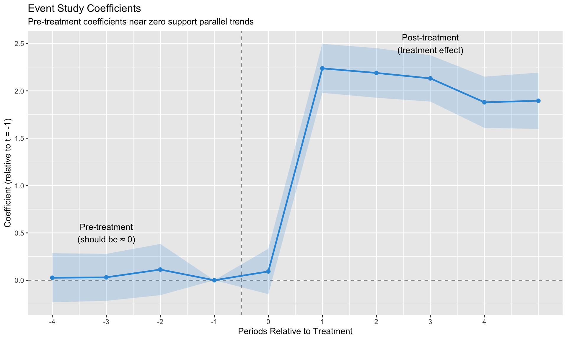
Pre-Trends Testing and Its Limits
The Event Study Specification
To assess parallel trends, estimate:
\[
Y_{it} = \alpha_i + \delta_t + \sum_{k \neq -1} \beta_k \cdot \mathbf{1}[t - T_i^* = k] + \varepsilon_{it}
\]
where \(T_i^*\) is the treatment time for unit \(i\), and \(k\) indexes relative time.
# Simulate event study with no pre-trends
es_data <- did_data %>%
  mutate(
    rel_time = time - T0,
    rel_time_fct = factor(rel_time)
  )

# Estimate event study
es_model <- feols(Y ~ i(rel_time_fct, treated, ref = "-1") | unit + time,
                   data = es_data, vcov = ~unit)

# Extract coefficients
coef_df <- data.frame(
  rel_time = as.numeric(gsub("rel_time_fct::(-?[0-9]+):treated", "\\1",
                              names(coef(es_model)))),
  estimate = coef(es_model),
  se = sqrt(diag(vcov(es_model)))
) %>%
  filter(!is.na(rel_time)) %>%
  mutate(
    lower = estimate - 1.96 * se,
    upper = estimate + 1.96 * se
  )

# Add reference period
coef_df <- bind_rows(
  coef_df,
  data.frame(rel_time = -1, estimate = 0, se = 0, lower = 0, upper = 0)
) %>%
  arrange(rel_time)

ggplot(coef_df, aes(x = rel_time, y = estimate)) +
  geom_hline(yintercept = 0, linetype = "dashed", alpha = 0.5) +
  geom_vline(xintercept = -0.5, linetype = "dashed", alpha = 0.5) +
  geom_ribbon(aes(ymin = lower, ymax = upper), alpha = 0.2, fill = "#3498db") +
  geom_line(color = "#3498db", size = 1) +
  geom_point(color = "#3498db", size = 2) +
  annotate("text", x = -3, y = 0.5, label = "Pre-treatment\n(should be ≈ 0)") +
  annotate("text", x = 3, y = 2.5, label = "Post-treatment\n(treatment effect)") +
  labs(title = "Event Study Coefficients",
       subtitle = "Pre-treatment coefficients near zero support parallel trends",
       x = "Periods Relative to Treatment",
       y = "Coefficient (relative to t = -1)") +
  scale_x_continuous(breaks = -4:4)
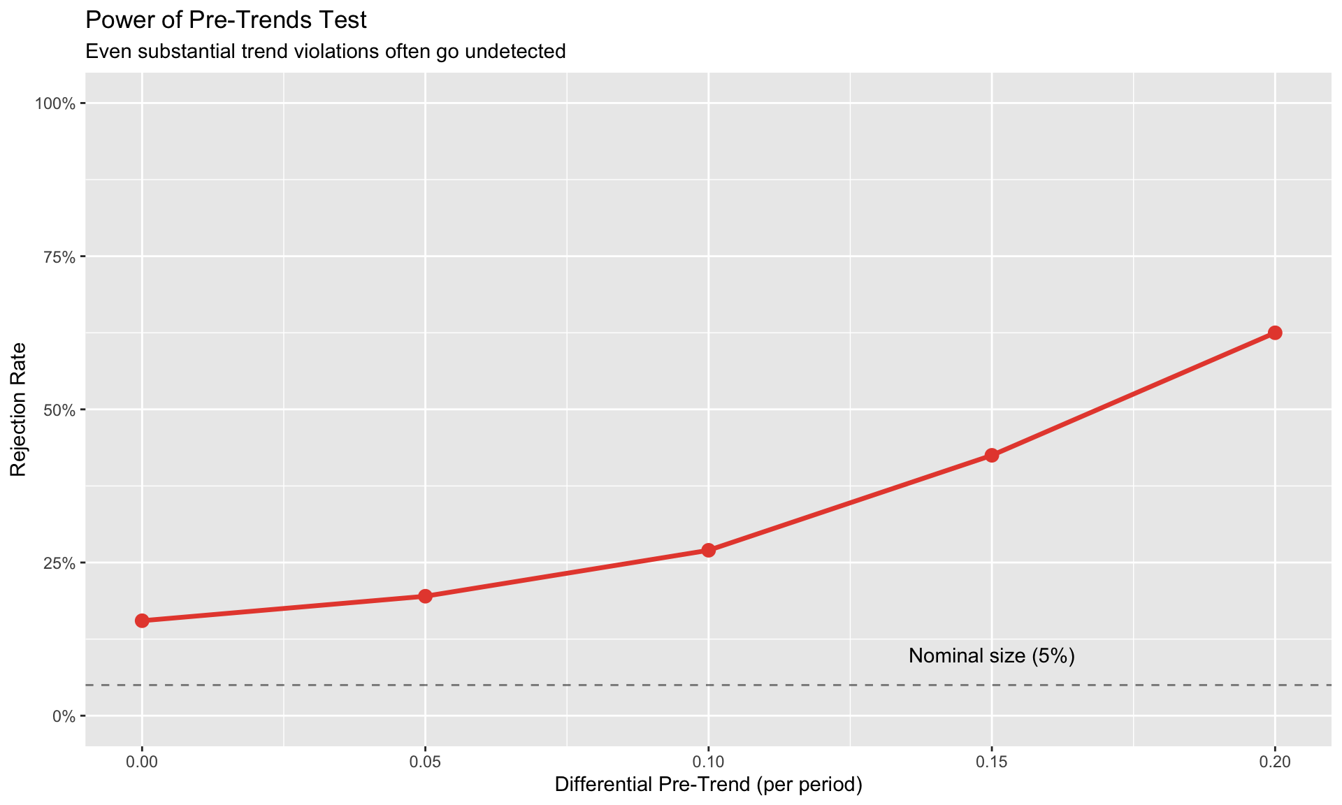
Roth (2022): Pre-Trends Testing Has Low Power
Passing a pre-trends test does NOT guarantee parallel trends hold. The test has low power against economically meaningful violations.
The problem: - Pre-trends tests are underpowered for typical sample sizes - Researchers often “shop” for specifications that pass the test - Even small pre-trends that pass the test can generate large bias
Quantifying the issue:
# Simulate: How often does pre-trend test miss a real violation?
simulate_pretrend_test <- function(delta_trend, n_sim = 500) {
  reject <- numeric(n_sim)

  for (s in 1:n_sim) {
    # Generate data with differential trend
    data <- expand.grid(unit = 1:50, time = 1:10) %>%
      mutate(
        treated = unit <= 25,
        post = time > 5,
        # Add differential trend for treated
        trend_effect = ifelse(treated, delta_trend * time, 0),
        Y = 2 + 0.3 * time + trend_effect +
            ifelse(treated, 1, 0) +
            ifelse(treated & post, 2, 0) +  # True effect = 2
            rnorm(n(), 0, 1)
      )

    # Test pre-trends (joint F-test on pre-treatment dummies)
    pre_data <- filter(data, time <= 5)
    model <- feols(Y ~ i(time, treated, ref = 5) | unit + time,
                   data = pre_data, vcov = ~unit)

    # Joint test of pre-treatment coefficients
    pre_coefs <- coef(model)[grep("time::", names(coef(model)))]
    if (length(pre_coefs) > 0) {
      # Simplified: check if any coefficient is significant
      reject[s] <- any(abs(pre_coefs) / sqrt(diag(vcov(model))[1:length(pre_coefs)]) > 1.96)
    }
  }

  mean(reject)  # Power = rejection rate
}

# Power against different trend violations
trend_violations <- c(0, 0.05, 0.1, 0.15, 0.2)
power <- sapply(trend_violations, simulate_pretrend_test, n_sim = 200)

power_df <- data.frame(
  differential_trend = trend_violations,
  power = power
)

ggplot(power_df, aes(x = differential_trend, y = power)) +
  geom_line(size = 1.2, color = "#e74c3c") +
  geom_point(size = 3, color = "#e74c3c") +
  geom_hline(yintercept = 0.05, linetype = "dashed", alpha = 0.5) +
  annotate("text", x = 0.15, y = 0.1, label = "Nominal size (5%)") +
  labs(title = "Power of Pre-Trends Test",
       subtitle = "Even substantial trend violations often go undetected",
       x = "Differential Pre-Trend (per period)",
       y = "Rejection Rate") +
  scale_y_continuous(labels = scales::percent, limits = c(0, 1))
Recommendations: 1. Report pre-trends but don’t over-interpret passing 2. Use sensitivity analysis (HonestDiD package) 3. Focus on institutional knowledge of why parallel trends should hold
Natural Experiments in Macro
The most credible DiD designs exploit exogenous shocks that affect some units but not others.
Examples of natural experiments: | Shock | Treatment | Control | Papers | |——-|———–|———|——–| | German reunification | East Germany | West Germany | Fuchs-Schündeln & Schündeln | | Swiss franc appreciation | Swiss border regions | French border regions | Auer et al. | | Oil price shocks | Oil importers vs exporters | — | Kilian & Lewis | | COVID-19 | High-exposure sectors | Low-exposure sectors | — |
What makes a good natural experiment: 1. Exogenous timing: Shock not driven by outcome of interest 2. Clear treatment/control: Units can be cleanly classified 3. No spillovers: Control units unaffected by treatment (SUTVA) 4. Plausible parallel trends: Pre-shock trends similar
Instrumental Variables
IV exploits exogenous variation to isolate the causal effect of an endogenous regressor.
The Logic of Instruments
An instrument \(Z\) satisfies:
1. Relevance: \(Z\) affects \(X\) \[
\text{Cov}(Z, X) \neq 0
\]
2. Exclusion: \(Z\) affects \(Y\) only through \(X\) \[
\text{Cov}(Z, \varepsilon) = 0
\]
Graphically:
Z → X → Y
Z ↛ Y (directly)
The IV estimator: \[
\hat{\beta}_{IV} = \frac{\text{Cov}(Z, Y)}{\text{Cov}(Z, X)} = \frac{\text{Reduced form}}{\text{First stage}}
\]
Two-Stage Least Squares
First stage: Regress \(X\) on \(Z\) and controls \[
X_{it} = \pi_0 + \pi_1 Z_{it} + W_{it}'\gamma + \nu_{it}
\]
Second stage: Regress \(Y\) on predicted \(\hat{X}\) and controls \[
Y_{it} = \beta_0 + \beta_1 \hat{X}_{it} + W_{it}'\delta + \varepsilon_{it}
\]
# Simulate IV setting
N <- 500
true_beta <- 0.5

# Instrument Z
Z <- rnorm(N)

# Endogenous X (correlated with error)
U <- rnorm(N)  # Unobserved confounder
X <- 0.7 * Z + 0.8 * U + rnorm(N, 0, 0.3)

# Outcome
Y <- true_beta * X + 0.6 * U + rnorm(N, 0, 0.5)

iv_data <- data.frame(Y = Y, X = X, Z = Z)

# OLS (biased)
ols_fit <- lm(Y ~ X, data = iv_data)

# IV
iv_fit <- feols(Y ~ 1 | X ~ Z, data = iv_data)

cat("True effect:", true_beta, "\n")
cat("OLS estimate:", round(coef(ols_fit)["X"], 3), "(biased upward due to U)\n")
OLS estimate: 0.895 (biased upward due to U)
cat("IV estimate:", round(coef(iv_fit)["fit_X"], 3), "(consistent)\n")
IV estimate: 0.591 (consistent)
cat("First-stage F:", round(fitstat(iv_fit, "ivf")$ivf1$stat, 1), "\n")
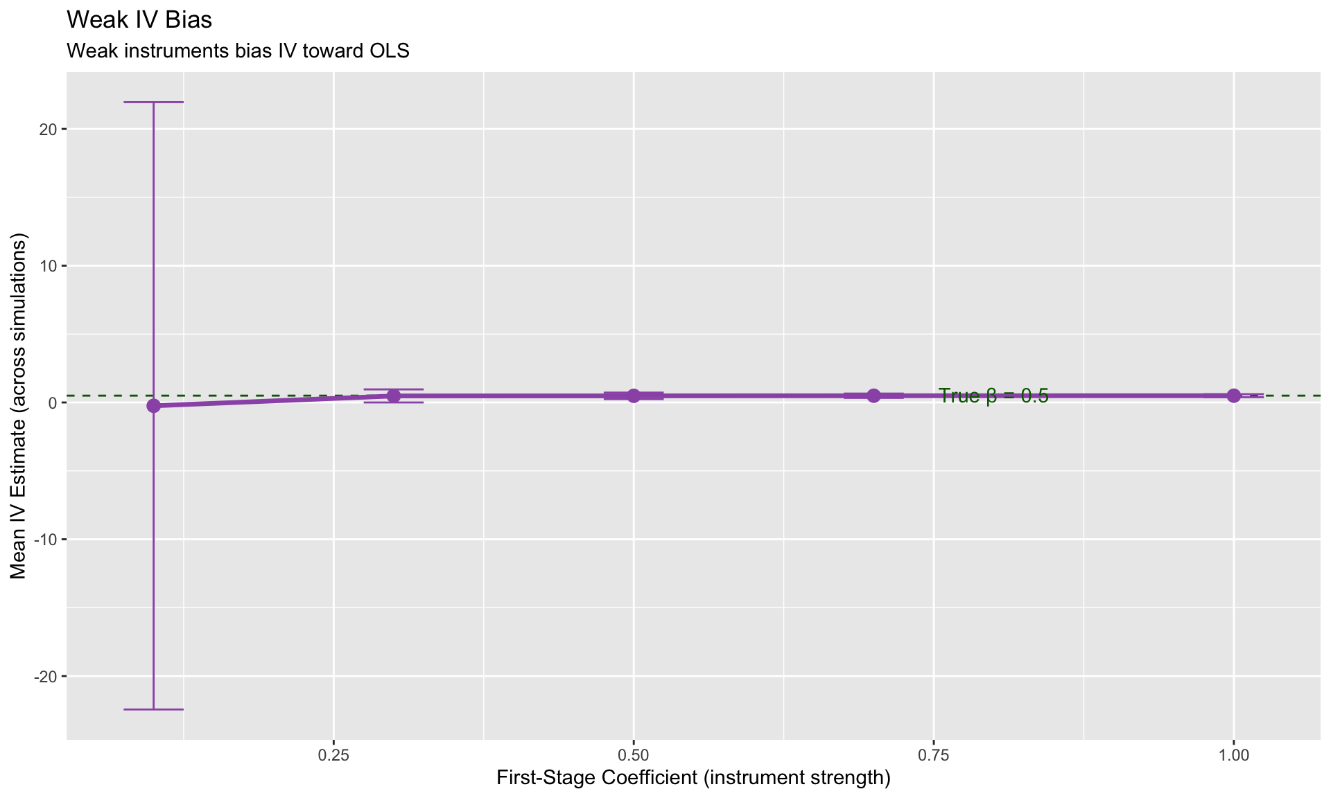
Weak Instruments
If the first stage is weak (\(\pi_1 \approx 0\)), IV estimates are: - Biased toward OLS - Have inflated standard errors - Unreliable inference
Rule of thumb: First-stage F-statistic > 10 (Stock & Yogo)
Diagnosis:
# Demonstrate weak IV bias
simulate_iv <- function(first_stage_strength, n_sim = 1000) {
  estimates <- numeric(n_sim)

  for (s in 1:n_sim) {
    Z <- rnorm(200)
    U <- rnorm(200)
    X <- first_stage_strength * Z + 0.8 * U + rnorm(200, 0, 0.5)
    Y <- 0.5 * X + 0.6 * U + rnorm(200, 0, 0.5)

    iv_fit <- feols(Y ~ 1 | X ~ Z, data = data.frame(Y, X, Z))
    estimates[s] <- coef(iv_fit)["fit_X"]
  }

  data.frame(
    first_stage = first_stage_strength,
    mean_estimate = mean(estimates),
    sd_estimate = sd(estimates)
  )
}

strengths <- c(0.1, 0.3, 0.5, 0.7, 1.0)
weak_iv_results <- do.call(rbind, lapply(strengths, simulate_iv, n_sim = 500))

ggplot(weak_iv_results, aes(x = first_stage, y = mean_estimate)) +
  geom_hline(yintercept = 0.5, linetype = "dashed", color = "darkgreen") +
  geom_line(size = 1.2, color = "#9b59b6") +
  geom_point(size = 3, color = "#9b59b6") +
  geom_errorbar(aes(ymin = mean_estimate - 1.96*sd_estimate,
                    ymax = mean_estimate + 1.96*sd_estimate),
                width = 0.05, color = "#9b59b6") +
  annotate("text", x = 0.8, y = 0.55, label = "True β = 0.5", color = "darkgreen") +
  labs(title = "Weak IV Bias",
       subtitle = "Weak instruments bias IV toward OLS",
       x = "First-Stage Coefficient (instrument strength)",
       y = "Mean IV Estimate (across simulations)")
Shift-Share (Bartik) Instruments
A common IV strategy in macro uses shift-share designs:
\[
Z_{it} = \sum_k s_{ik,0} \cdot g_{kt}
\]
where: - \(s_{ik,0}\) = pre-period share of sector \(k\) in unit \(i\) - \(g_{kt}\) = national/global shock to sector \(k\) at time \(t\)
Example: China shock (Autor, Dorn, Hanson 2013) - \(s_{ik}\) = share of industry \(k\) in region \(i\)’s employment - \(g_{kt}\) = growth of Chinese imports in industry \(k\)
Identification can come from: - Exogeneity of shares (Goldsmith-Pinkham, Sorkin & Swift 2020) - Exogeneity of shocks (Borusyak, Hull & Jaravel 2022)
GMM for Dynamic Panels
When the model includes lagged dependent variables:
\[
Y_{it} = \rho Y_{i,t-1} + X_{it}'\beta + \alpha_i + \varepsilon_{it}
\]
Standard FE is biased (Nickell bias): \(\text{plim}(\hat{\rho}_{FE}) = \rho - \frac{1+\rho}{T-1}\)
Solutions:
| Anderson-Hsiao |
\(Y_{i,t-2}\) |
Simple, conservative |
| Arellano-Bond (diff-GMM) |
\(Y_{i,t-2}, Y_{i,t-3}, ...\) |
Moderately persistent \(Y\) |
| Blundell-Bond (sys-GMM) |
Add levels equations |
Highly persistent \(Y\) |
With \(T = 84\) quarters and \(\rho = 0.9\), the bias is approximately \(\frac{1.9}{83} \approx 2.3\%\). For long panels, FE may be acceptable.
Small-Sample Inference
Standard asymptotic inference fails with few clusters. This section covers robust alternatives.
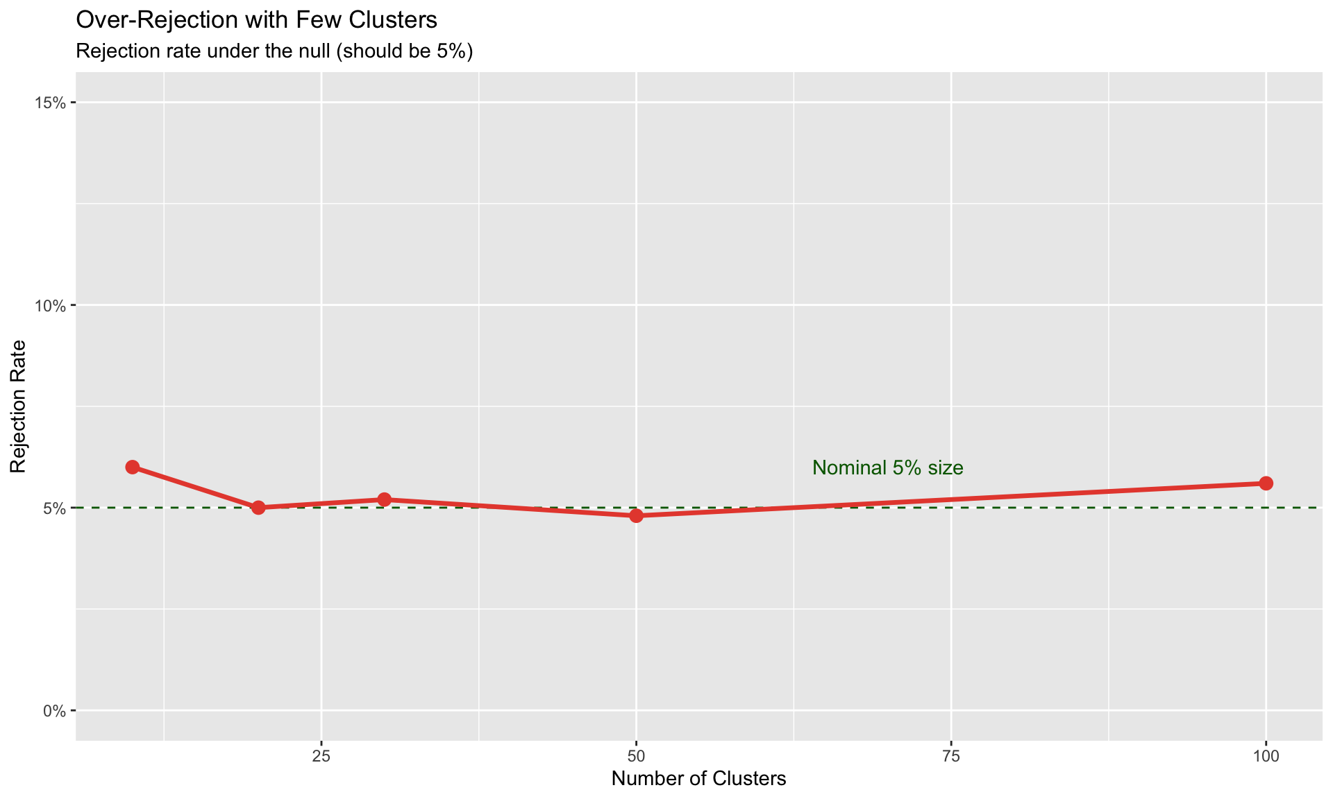
The Small-Cluster Problem
Cluster-robust standard errors assume \(G \to \infty\) (number of clusters goes to infinity).
With \(G < 50\) clusters: - Standard errors are biased downward - t-statistics are inflated - Rejection rates exceed nominal size
# Simulate rejection rates with different cluster sizes
simulate_rejection <- function(n_clusters, n_sim = 1000) {
  rejections <- 0

  for (s in 1:n_sim) {
    # Generate clustered data with NO true effect
    cluster_effects <- rnorm(n_clusters, 0, 2)

    data <- data.frame(
      cluster = rep(1:n_clusters, each = 10),
      cluster_effect = rep(cluster_effects, each = 10)
    ) %>%
      mutate(
        X = rnorm(n()) + cluster_effect * 0.3,
        Y = cluster_effect + rnorm(n())  # No effect of X!
      )

    # Test with clustered SEs
    fit <- feols(Y ~ X | cluster, data = data, vcov = ~cluster)
    p_value <- 2 * (1 - pt(abs(coef(fit)["X"] / se(fit)["X"]), df = n_clusters - 1))
    rejections <- rejections + (p_value < 0.05)
  }

  rejections / n_sim
}

cluster_sizes <- c(10, 20, 30, 50, 100)
rejection_rates <- sapply(cluster_sizes, simulate_rejection, n_sim = 500)

rej_df <- data.frame(clusters = cluster_sizes, rejection = rejection_rates)

ggplot(rej_df, aes(x = clusters, y = rejection)) +
  geom_hline(yintercept = 0.05, linetype = "dashed", color = "darkgreen") +
  geom_line(size = 1.2, color = "#e74c3c") +
  geom_point(size = 3, color = "#e74c3c") +
  annotate("text", x = 70, y = 0.06, label = "Nominal 5% size", color = "darkgreen") +
  labs(title = "Over-Rejection with Few Clusters",
       subtitle = "Rejection rate under the null (should be 5%)",
       x = "Number of Clusters",
       y = "Rejection Rate") +
  scale_y_continuous(labels = scales::percent, limits = c(0, 0.15))
Wild Cluster Bootstrap
The wild cluster bootstrap (Cameron, Gelbach & Miller 2008) provides valid inference with few clusters.
Algorithm: 1. Estimate the model, get residuals \(\hat{\varepsilon}_{it}\) 2. For \(b = 1, ..., B\): - Draw cluster-level weights \(w_g \in \{-1, +1\}\) (Rademacher) - Construct bootstrap outcome: \(Y^*_{it} = \hat{Y}_{it} + w_{g(i)} \cdot \hat{\varepsilon}_{it}\) - Re-estimate model, save t-statistic \(t^*_b\) 3. Compare actual t-statistic to bootstrap distribution
# Demonstrate wild cluster bootstrap (manual implementation)
# In practice, use fwildclusterboot::boottest()

# Generate data with few clusters
n_clusters <- 20
cluster_effects <- rnorm(n_clusters, 0, 2)

wcb_data <- data.frame(
  cluster = rep(1:n_clusters, each = 15),
  cluster_effect = rep(cluster_effects, each = 15)
) %>%
  mutate(
    X = rnorm(n()) + cluster_effect * 0.3,
    Y = 0.5 * X + cluster_effect + rnorm(n(), 0, 0.8)  # True effect = 0.5
  )

# Standard estimation
model <- feols(Y ~ X | cluster, data = wcb_data, vcov = ~cluster)

cat("=== Standard Cluster-Robust Inference ===\n")
=== Standard Cluster-Robust Inference ===
cat("Estimate:", round(coef(model)["X"], 3), "\n")
cat("Cluster SE:", round(se(model)["X"], 3), "\n")
cat("t-stat:", round(coef(model)["X"] / se(model)["X"], 2), "\n")
cat("p-value (t-dist, df =", n_clusters - 1, "):",
    round(2 * pt(-abs(coef(model)["X"] / se(model)["X"]), df = n_clusters - 1), 4), "\n\n")
p-value (t-dist, df = 19 ): 0
# Manual wild cluster bootstrap implementation
wild_cluster_bootstrap <- function(model, data, cluster_var, B = 999) {
  # Get model components
  y_fitted <- fitted(model)
  resid <- residuals(model)
  clusters <- unique(data[[cluster_var]])
  G <- length(clusters)

  # Original t-statistic
  t_orig <- coef(model)["X"] / se(model)["X"]

  # Bootstrap
  t_boot <- numeric(B)
  for (b in 1:B) {
    # Rademacher weights (cluster-level)
    weights <- sample(c(-1, 1), G, replace = TRUE)
    names(weights) <- clusters

    # Construct bootstrap outcome
    data$Y_boot <- y_fitted + weights[as.character(data[[cluster_var]])] * resid

    # Re-estimate under null (impose beta = 0)
    model_boot <- feols(Y_boot ~ X | cluster, data = data, vcov = ~cluster)
    t_boot[b] <- coef(model_boot)["X"] / se(model_boot)["X"]
  }

  # Two-sided p-value
  p_value <- mean(abs(t_boot) >= abs(t_orig))

  list(t_orig = t_orig, t_boot = t_boot, p_value = p_value)
}

# Run bootstrap (reduced B for speed)
boot_result <- wild_cluster_bootstrap(model, wcb_data, "cluster", B = 499)

cat("=== Wild Cluster Bootstrap (Manual) ===\n")
=== Wild Cluster Bootstrap (Manual) ===
cat("Bootstrap p-value:", round(boot_result$p_value, 4), "\n")
Bootstrap p-value: 0.5291
cat("(In practice, use fwildclusterboot::boottest() for efficiency)\n")
(In practice, use fwildclusterboot::boottest() for efficiency)
When to Use What
| G > 50 |
Standard cluster-robust SE |
vcov = ~cluster |
| 30 < G < 50 |
t-distribution with G-1 df |
vcov = ~cluster + manual df adjustment |
| 10 < G < 30 |
Wild cluster bootstrap |
fwildclusterboot::boottest() |
| G < 10 |
Randomization inference |
Permutation tests |
With G < 10, use Webb (6-point) weights instead of Rademacher:
boottest(model, param = "X", clustid = "cluster", type = "webb")
Putting It Together
Checklist for Identification
Before claiming a causal effect, verify:
- What is the source of identifying variation?
- Within-unit over time? (FE)
- Across units hit by shock? (DiD)
- Exogenous instrument? (IV)
- What assumptions does this require?
- Parallel trends? (DiD)
- Exclusion restriction? (IV)
- No anticipation? (Event study)
- What are the threats?
- Time-varying confounders?
- Spillovers to control group?
- Weak instruments?
- What robustness checks support the design?
- Pre-trends (with caveats about power)
- Placebo tests
- Alternative control groups
- Sensitivity analysis
Common Pitfalls
| Overinterpreting pre-trends |
Low power against violations |
Use HonestDiD, report sensitivity |
| Post-treatment controls |
Blocks causal path |
Only control for pre-determined variables |
| Weak instruments |
Bias toward OLS |
Report first-stage F, use robust methods |
| Few clusters |
Over-rejection |
Wild cluster bootstrap |
| Staggered treatment |
TWFE bias |
Callaway-Sant’Anna, Sun-Abraham |
| Anticipation effects |
Violates sharp treatment timing |
Test for pre-treatment effects |
Frequently Asked Questions
How do I know if parallel trends holds?
You can’t prove it—it’s about counterfactuals we don’t observe. You can: - Show pre-trends are flat (but low power—Roth 2022) - Argue institutionally why the assumption is plausible - Run sensitivity analysis (HonestDiD) - Find a better control group
When should I use IV vs. DiD?
Use DiD when: - You have a clear treatment/control distinction - Treatment timing is plausibly exogenous - Parallel trends is defensible
Use IV when: - Treatment varies continuously (not just on/off) - You have a plausibly exogenous source of variation in treatment - Exclusion restriction is defensible
What if my first-stage F is below 10?
Options: 1. Find a stronger instrument 2. Use weak-IV robust methods (Anderson-Rubin, LIML) 3. Report reduced form instead (effect of Z on Y) 4. Interpret results as a lower bound (if bias direction is known)
How many clusters do I need?
- 50+ clusters: Standard cluster-robust SEs are fine
- 30-50 clusters: Use t-distribution with G-1 df
- 10-30 clusters: Wild cluster bootstrap
- <10 clusters: Randomization inference, or aggregate to higher level
Summary
Key takeaways from this module:
Correlation ≠ causation due to simultaneity, selection, and omitted variables
Controlling for observables doesn’t solve endogeneity from unobservables
DiD exploits discrete shocks but requires parallel trends—a strong, untestable assumption
Pre-trends tests have low power—passing doesn’t guarantee validity
IV isolates exogenous variation but requires a valid instrument (relevant + excludable)
Small clusters require wild cluster bootstrap for valid inference
Next: Module 3: Local Projections