Synthetic Control Methods

Data-Driven Counterfactuals for Comparative Case Studies

When DiD Fails

Difference-in-differences requires parallel trends—the assumption that treated and control groups would have followed similar paths absent treatment. But what happens when:

• You have only one treated unit?
• No control unit has trends parallel to the treated unit?
• The treated unit is unique (e.g., West Germany, California, a specific country)?

Synthetic Control Methods (SCM) solve this by constructing a weighted combination of untreated units that together replicate the treated unit’s pre-treatment trajectory. Instead of assuming parallel trends, SCM matches them.

The Core Insight

Method	Comparison Unit	Key Assumption
DiD	Actual control group	Parallel trends
SCM	Synthetic control (weighted donors)	Weights match pre-treatment outcomes

SCM is transparent: you see exactly which units contribute to the counterfactual and with what weights.

The SCM Framework

Abadie, Diamond & Hainmueller (2010, 2015)

Setup and Notation

Following the foundational papers:

\[ \begin{aligned} &\text{Treated unit: } i = 1 \\ &\text{Donor pool: } i = 2, \ldots, J+1 \\ &\text{Pre-treatment: } t = 1, \ldots, T_0 \\ &\text{Post-treatment: } t = T_0+1, \ldots, T \end{aligned} \]

We want to estimate the treatment effect: \[ \tau_{1t} = Y_{1t}(1) - Y_{1t}(0) \quad \text{for } t > T_0 \]

We observe \(Y_{1t}(1)\) (the actual outcome under treatment). The challenge is estimating \(Y_{1t}(0)\)—what would have happened without treatment.

The Synthetic Control Estimator

Find weights \(W^* = (w_2, \ldots, w_{J+1})'\) that solve:

\[ \min_W \|X_1 - X_0 W\|_V \quad \text{subject to } w_j \geq 0, \sum_{j=2}^{J+1} w_j = 1 \]

where:

• \(X_1\) = vector of pre-treatment characteristics of treated unit
• \(X_0\) = matrix of pre-treatment characteristics of donor units
• \(V\) = diagonal weight matrix (predictor importance)
• Constraints ensure weights are non-negative and sum to one (convex combination)

The synthetic control outcome: \[ \hat{Y}_{1t}(0) = \sum_{j=2}^{J+1} w_j^* Y_{jt} \]

The treatment effect estimate: \[ \hat{\tau}_{1t} = Y_{1t} - \sum_{j=2}^{J+1} w_j^* Y_{jt} \]

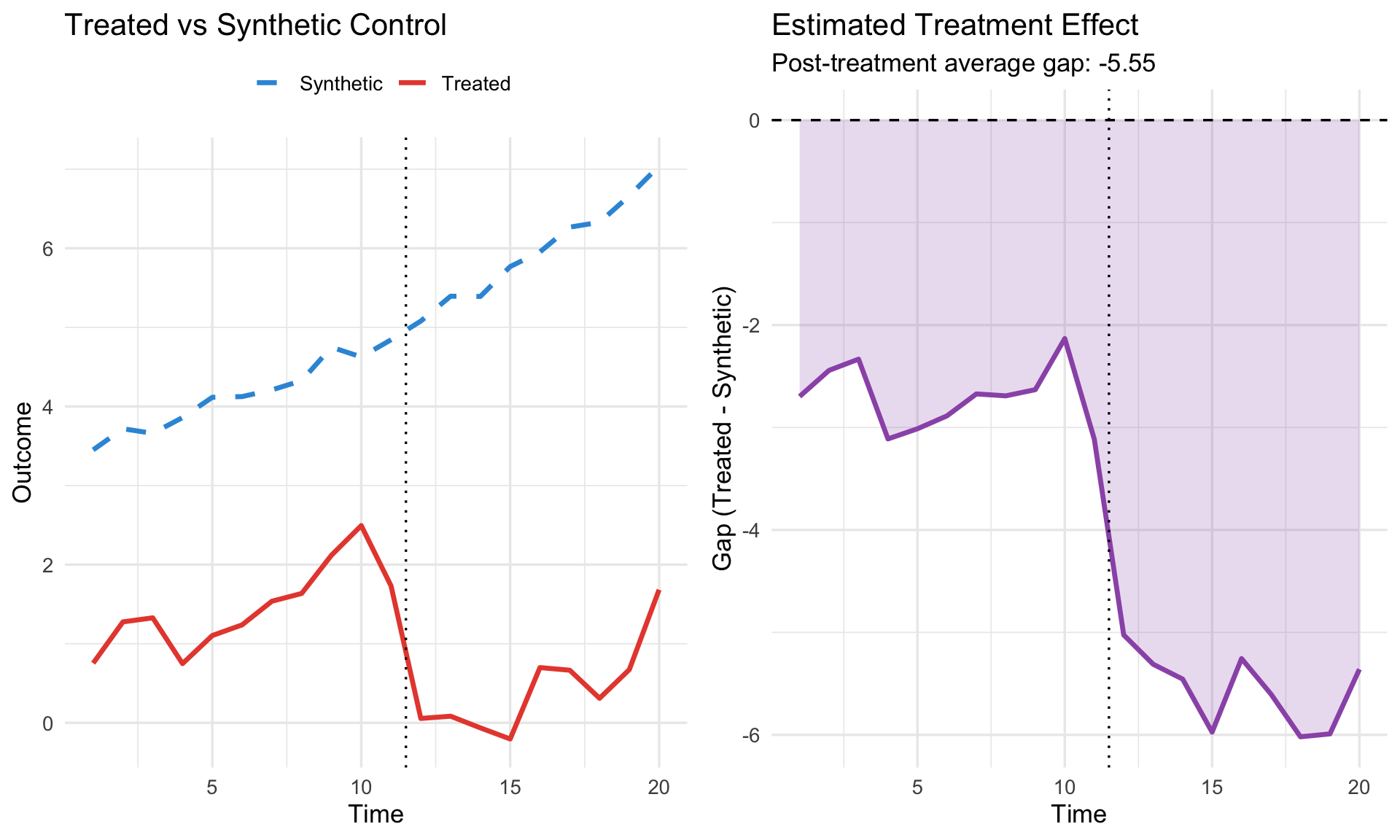
# Simulate SCM scenario
set.seed(123)
T_total <- 20
T0 <- 12  # Treatment after period 12

# Treated unit trajectory
treated_base <- cumsum(c(0, rnorm(T0-1, 0.3, 0.2)))
treated_post <- treated_base[T0] + cumsum(rnorm(T_total - T0, -0.1, 0.25))
treated <- c(treated_base, treated_post)

# Donor units (5 potential controls)
donors <- lapply(1:5, function(i) {
  base <- cumsum(c(0, rnorm(T_total-1, 0.25 + 0.05*i, 0.3)))
  data.frame(time = 1:T_total, unit = paste("Donor", i), y = base)
}) %>% bind_rows()

# Optimal weights (illustrative - found to match pre-treatment)
weights <- c(0.45, 0.30, 0.15, 0.10, 0.00)

# Construct synthetic control
synthetic <- donors %>%
  mutate(weight = case_when(
    unit == "Donor 1" ~ weights[1],
    unit == "Donor 2" ~ weights[2],
    unit == "Donor 3" ~ weights[3],
    unit == "Donor 4" ~ weights[4],
    TRUE ~ weights[5]
  )) %>%
  group_by(time) %>%
  summarize(y = sum(y * weight), .groups = "drop")

# Combine for plotting
treated_df <- data.frame(time = 1:T_total, y = treated, unit = "Treated")

ggplot() +
  # Donor units (faded)
  geom_line(data = donors, aes(x = time, y = y, group = unit),
            color = "gray70", alpha = 0.4, linewidth = 0.7) +
  # Synthetic control
  geom_line(data = synthetic, aes(x = time, y = y),
            color = "#3498db", linewidth = 1.3, linetype = "dashed") +
  # Treated unit
  geom_line(data = treated_df, aes(x = time, y = y),
            color = "#e74c3c", linewidth = 1.3) +
  # Treatment line
  geom_vline(xintercept = T0 + 0.5, linetype = "dotted", alpha = 0.7) +
  annotate("text", x = T0 + 1, y = max(treated) * 0.95,
           label = "Treatment", hjust = 0, size = 3.5) +
  # Gap annotation
  annotate("segment", x = T_total - 1, xend = T_total - 1,
           y = treated[T_total-1], yend = synthetic$y[T_total-1],
           arrow = arrow(ends = "both", length = unit(0.08, "inches")),
           color = "#9b59b6", linewidth = 1) +
  annotate("text", x = T_total - 0.5,
           y = mean(c(treated[T_total-1], synthetic$y[T_total-1])),
           label = expression(hat(tau)), hjust = 0, size = 4, color = "#9b59b6") +
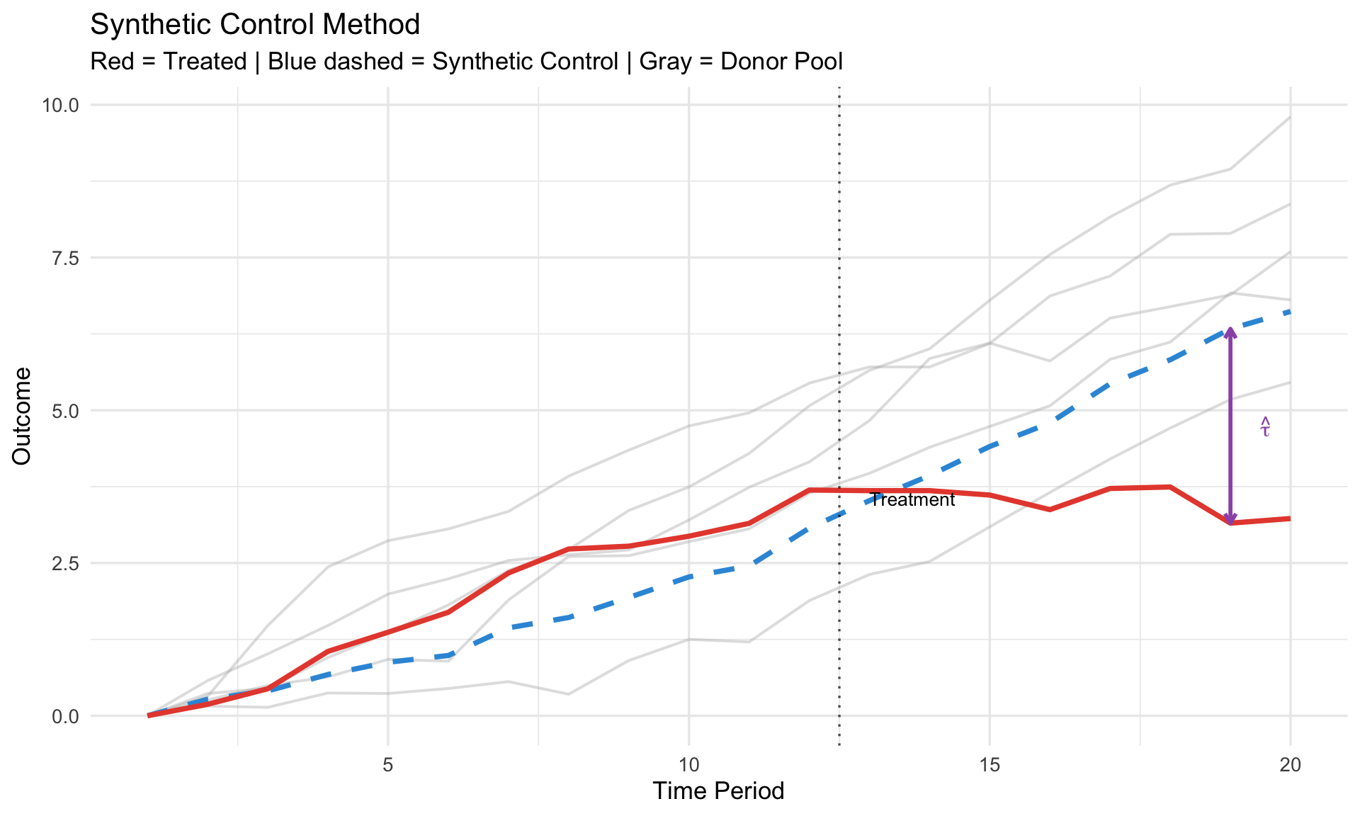
  labs(title = "Synthetic Control Method",
       subtitle = "Red = Treated | Blue dashed = Synthetic Control | Gray = Donor Pool",
       x = "Time Period", y = "Outcome") +
  theme(legend.position = "none")

Synthetic control: construct counterfactual from weighted donors

Choosing Predictors (\(X\))

The predictor matrix \(X\) typically includes:

Predictor Type	Examples	Rationale
Pre-treatment outcomes	\(Y_{1,T_0}, Y_{1,T_0-1}, \ldots\)	Forces trajectory matching
Economic fundamentals	GDP growth, inflation, trade openness	Structural similarity
Demographics	Population, urbanization	Background comparability
Policy variables	Tax rates, regulations	Institutional similarity

ImportantInclude Pre-Treatment Outcomes

Abadie (2021) emphasizes: always include multiple pre-treatment outcomes as predictors. This forces the synthetic control to track the actual trajectory, not just match averages.

The Nested Optimization

In practice, SCM solves two nested problems:

Inner problem (given predictor weights \(V\)): \[ W^*(V) = \arg\min_W (X_1 - X_0 W)' V (X_1 - X_0 W) \]

Outer problem (choose \(V\) to minimize pre-treatment fit): \[ V^* = \arg\min_V \sum_{t=1}^{T_0} \left(Y_{1t} - \sum_{j} w_j^*(V) Y_{jt}\right)^2 \]

This ensures the weights are chosen to match the outcome trajectory, not just predictor averages.

Inference: Permutation Tests

With one treated unit, standard inference doesn’t apply. SCM uses permutation-based inference.

The Placebo Test

Idea: Apply SCM to each donor unit as if it were treated. If the treated unit’s effect is real, its gap should be unusually large compared to placebo gaps.

Procedure:

1. Estimate SCM for treated unit → get gap \(\hat{\tau}_{1t}\)
2. For each donor \(j = 2, \ldots, J+1\):
   • Pretend unit \(j\) is treated (remove from donor pool)
   • Construct synthetic control from remaining units
   • Calculate placebo gap \(\hat{\tau}_{jt}\)
3. Compare: Is \(|\hat{\tau}_{1t}|\) extreme relative to \(\{|\hat{\tau}_{jt}|\}\)?

P-value: \[ p = \frac{\#\{j : |\hat{\tau}_j| \geq |\hat{\tau}_1|\}}{J + 1} \]

# Simulate placebo test
set.seed(789)
n_placebo <- 12

# Treated unit has real effect
treated_gap <- c(rep(0, T0), cumsum(rnorm(T_total - T0, -0.5, 0.2)))

# Placebo gaps (no real effect)
placebo_gaps <- lapply(1:n_placebo, function(i) {
  gap <- c(rnorm(T0, 0, 0.25), rnorm(T_total - T0, 0, 0.35))
  data.frame(time = 1:T_total, gap = gap, unit = paste("Placebo", i))
}) %>% bind_rows()

# Combine
all_gaps <- bind_rows(
  data.frame(time = 1:T_total, gap = treated_gap, unit = "Treated"),
  placebo_gaps
)

ggplot(all_gaps, aes(x = time, y = gap, group = unit)) +
  geom_line(data = filter(all_gaps, unit != "Treated"),
            color = "gray60", alpha = 0.5, linewidth = 0.6) +
  geom_line(data = filter(all_gaps, unit == "Treated"),
            color = "#e74c3c", linewidth = 1.3) +
  geom_hline(yintercept = 0, linetype = "dashed", alpha = 0.5) +
  geom_vline(xintercept = T0 + 0.5, linetype = "dotted", alpha = 0.7) +
  annotate("text", x = 2, y = min(all_gaps$gap) * 0.8,
           label = "Gray = Placebo gaps\nRed = Treated unit gap",
           hjust = 0, size = 3, color = "gray40") +
  labs(title = "Placebo Test for Inference",
       subtitle = "If treatment effect is real, treated unit's gap should be extreme",
       x = "Time Period", y = "Gap (Actual - Synthetic)")

Placebo test: treated unit gap vs. placebo distribution

RMSPE Ratio

To account for pre-treatment fit quality, use the RMSPE ratio:

\[ \text{Ratio}_j = \frac{\text{RMSPE}_{j,\text{post}}}{\text{RMSPE}_{j,\text{pre}}} \]

where: \[ \text{RMSPE}_{j,\text{pre}} = \sqrt{\frac{1}{T_0} \sum_{t=1}^{T_0} (Y_{jt} - \hat{Y}_{jt}^{\text{synth}})^2} \]

Rationale: A unit with poor pre-treatment fit may have large post-treatment gaps just from noise. The ratio normalizes by pre-treatment fit quality.

# Calculate RMSPE ratios
rmspe_pre <- c(0.12, runif(n_placebo, 0.15, 0.6))  # Treated has good fit
rmspe_post <- c(1.8, runif(n_placebo, 0.2, 1.2))   # Treated has large post gap

rmspe_df <- data.frame(
  unit = c("Treated", paste("Placebo", 1:n_placebo)),
  rmspe_pre = rmspe_pre,
  rmspe_post = rmspe_post
) %>%
  mutate(
    ratio = rmspe_post / rmspe_pre,
    is_treated = unit == "Treated"
  ) %>%
  arrange(desc(ratio))

# P-value
p_val <- mean(rmspe_df$ratio >= rmspe_df$ratio[rmspe_df$unit == "Treated"])

ggplot(rmspe_df, aes(x = reorder(unit, ratio), y = ratio, fill = is_treated)) +
  geom_col(width = 0.7) +
  geom_hline(yintercept = rmspe_df$ratio[rmspe_df$unit == "Treated"],
             linetype = "dashed", color = "#e74c3c", linewidth = 0.8) +
  coord_flip() +
  scale_fill_manual(values = c("FALSE" = "#bdc3c7", "TRUE" = "#e74c3c")) +
  labs(title = "RMSPE Ratio Distribution",
       subtitle = paste0("Treated unit ratio = ",
                        round(rmspe_df$ratio[rmspe_df$unit == "Treated"], 1),
                        " | Implied p-value = ", round(p_val, 3)),
       x = "", y = "Post/Pre RMSPE Ratio") +
  theme(legend.position = "none")

RMSPE ratio: normalizing by pre-treatment fit

Synthetic Difference-in-Differences

Arkhangelsky et al. (2021)

Synthetic DiD combines the strengths of SCM and DiD:

Method	Handles Multiple Treated?	Requires Parallel Trends?
DiD	Yes	Yes
SCM	No (designed for one)	No (matches trajectories)
Synthetic DiD	Yes	No

The Estimator

Synthetic DiD finds:

1. Unit weights \(\omega_i\) (like SCM) — make controls look like treated pre-treatment
2. Time weights \(\lambda_t\) (novel) — emphasize pre-treatment periods that predict post-treatment

\[ \hat{\tau}^{sdid} = \left(\bar{Y}_{tr,post}^{\omega} - \bar{Y}_{co,post}^{\omega}\right) - \left(\bar{Y}_{tr,pre}^{\lambda} - \bar{Y}_{co,pre}^{\omega,\lambda}\right) \]

The optimization: \[ \min_{\omega, \lambda} \sum_{i: \text{control}} \sum_{t \leq T_0} \left(Y_{it} - \lambda_t - \omega_i - \mu\right)^2 + \text{regularization} \]

Advantages

1. Works with multiple treated units (unlike classic SCM)
2. Doesn’t require exact pre-treatment match (unlike SCM)
3. Doesn’t require parallel trends (unlike DiD)
4. Doubly robust: consistent if either unit OR time weights are correct

# Illustrate multiple treated units scenario
sdid_data <- expand.grid(
  time = 1:15,
  unit = 1:8
) %>%
  mutate(
    treated = unit <= 3,
    post = time > 10,
    treatment = treated & post,
    # Generate outcomes
    unit_fe = unit * 0.4,
    time_trend = 0.2 * time,
    tau = ifelse(treatment, 2, 0),
    y = unit_fe + time_trend + tau + rnorm(n(), 0, 0.4),
    group = ifelse(treated, "Treated (3 units)", "Control (5 units)")
  )

# Aggregate by group
agg_data <- sdid_data %>%
  group_by(time, group) %>%
  summarize(y = mean(y), .groups = "drop")

ggplot(agg_data, aes(x = time, y = y, color = group)) +
  geom_line(linewidth = 1.2) +
  geom_vline(xintercept = 10.5, linetype = "dashed", alpha = 0.5) +
  scale_color_manual(values = c("Control (5 units)" = "#3498db",
                                 "Treated (3 units)" = "#e74c3c")) +
  annotate("text", x = 11, y = max(agg_data$y) * 0.95,
           label = "Treatment", hjust = 0, size = 3.5) +
  labs(title = "Synthetic DiD: Multiple Treated Units",
       subtitle = "Synthetic DiD reweights controls to match treated pre-treatment trajectory",
       x = "Time", y = "Average Outcome",
       color = "") +
  theme(legend.position = "top")

Synthetic DiD handles multiple treated units

Implementation in R

Using augsynth Package

The augsynth package by Ben-Michael et al. implements augmented synthetic control, which combines SCM with outcome modeling (Ridge regression) for improved finite-sample performance.

library(augsynth)

# Basic synthetic control
syn <- augsynth(
  outcome ~ treatment | covariate1 + covariate2,  # outcome ~ treatment | predictors
  unit = unit_id,
  time = time_id,
  data = panel_data,
  t_int = treatment_time,    # when treatment begins
  progfunc = "Ridge"         # augmentation: "None", "Ridge", "EN"
)

# Results
summary(syn)
plot(syn)

# Extract weights
syn$weights

Key Arguments

Argument	Description
progfunc	Augmentation method: "None" (pure SCM), "Ridge", "EN" (elastic net)
t_int	Treatment time (integer or date)
fixedeff	Include unit fixed effects in augmentation?

Multiple Treated Units with multisynth

# When multiple units are treated (possibly at different times)
multi_syn <- multisynth(
  outcome ~ treatment | covariates,
  unit = unit_id,
  time = time_id,
  data = panel_data,
  n_leads = 8,      # post-treatment horizons to estimate
  n_lags = 4        # pre-treatment periods to match
)

summary(multi_syn)
plot(multi_syn)

Using synthdid Package

The synthdid package by Arkhangelsky et al. implements Synthetic Difference-in-Differences.

library(synthdid)

# Prepare data as matrices
# Y: units × time matrix of outcomes
Y <- panel_data %>%
  pivot_wider(id_cols = unit, names_from = time, values_from = outcome) %>%
  column_to_rownames("unit") %>%
  as.matrix()

# W: units × time matrix of treatment indicators (1 if treated)
W <- panel_data %>%
  pivot_wider(id_cols = unit, names_from = time, values_from = treated) %>%
  column_to_rownames("unit") %>%
  as.matrix()

# Synthetic DiD estimate
tau_sdid <- synthdid_estimate(Y, W)

# Standard error (placebo-based)
se_sdid <- sqrt(vcov(tau_sdid, method = "placebo"))

# Compare to pure SC and pure DiD
tau_sc <- sc_estimate(Y, W)
tau_did <- did_estimate(Y, W)

# Visualize
synthdid_plot(tau_sdid)

Worked Example

# Create synthetic panel data for demonstration
set.seed(42)
n_units <- 15
n_periods <- 20
treatment_time <- 12

# Unit 1 is treated
panel <- expand.grid(
  unit = 1:n_units,
  time = 1:n_periods
) %>%
  mutate(
    treated_unit = (unit == 1),
    post = (time >= treatment_time),
    treatment = treated_unit & post,
    # Pre-treatment characteristics
    x1 = rnorm(n(), mean = unit/5, sd = 0.3),
    x2 = rnorm(n(), mean = time/10, sd = 0.2),
    # Outcome with treatment effect for unit 1
    unit_fe = unit * 0.5,
    time_fe = 0.15 * time,
    tau = ifelse(treatment, -2.5 - 0.1*(time - treatment_time), 0),
    y = unit_fe + time_fe + 0.3*x1 + 0.2*x2 + tau + rnorm(n(), 0, 0.4)
  )

# --- Manual SCM Implementation ---

# Pre-treatment data
pre_data <- panel %>% filter(time < treatment_time)

# Treated unit pre-treatment outcomes
y_treated_pre <- pre_data %>%
  filter(unit == 1) %>%
  arrange(time) %>%
  pull(y)

# Donor pre-treatment outcomes (matrix: time × donors)
Y_donors_pre <- pre_data %>%
  filter(unit != 1) %>%
  pivot_wider(id_cols = time, names_from = unit, values_from = y) %>%
  arrange(time) %>%
  select(-time) %>%
  as.matrix()

# Find weights via constrained least squares (simplified)
# In practice, use quadprog or augsynth
# Here: OLS projection then normalize positive weights

weights_raw <- coef(lm(y_treated_pre ~ Y_donors_pre - 1))
weights_raw[is.na(weights_raw) | weights_raw < 0] <- 0
weights <- weights_raw / sum(weights_raw)

# Construct synthetic control for all periods
synthetic <- panel %>%
  filter(unit != 1) %>%
  left_join(
    data.frame(unit = 2:n_units, weight = weights),
    by = "unit"
  ) %>%
  group_by(time) %>%
  summarize(y_synth = sum(y * weight, na.rm = TRUE), .groups = "drop")

# Get treated outcomes
treated_outcomes <- panel %>%
  filter(unit == 1) %>%
  select(time, y_treated = y)

# Calculate gaps
results <- left_join(treated_outcomes, synthetic, by = "time") %>%
  mutate(gap = y_treated - y_synth)

# --- Visualization ---

p1 <- ggplot(results, aes(x = time)) +
  geom_line(aes(y = y_treated, color = "Treated"), linewidth = 1.2) +
  geom_line(aes(y = y_synth, color = "Synthetic"), linewidth = 1.2, linetype = "dashed") +
  geom_vline(xintercept = treatment_time - 0.5, linetype = "dotted") +
  scale_color_manual(values = c("Treated" = "#e74c3c", "Synthetic" = "#3498db")) +
  labs(title = "Treated vs Synthetic Control",
       x = "Time", y = "Outcome", color = "") +
  theme(legend.position = "top")

p2 <- ggplot(results, aes(x = time, y = gap)) +
  geom_line(linewidth = 1.2, color = "#9b59b6") +
  geom_ribbon(aes(ymin = pmin(0, gap), ymax = pmax(0, gap)),
              fill = "#9b59b6", alpha = 0.2) +
  geom_hline(yintercept = 0, linetype = "dashed") +
  geom_vline(xintercept = treatment_time - 0.5, linetype = "dotted") +
  labs(title = "Estimated Treatment Effect",
       subtitle = paste0("Post-treatment average gap: ",
                        round(mean(results$gap[results$time >= treatment_time]), 2)),
       x = "Time", y = "Gap (Treated - Synthetic)")

gridExtra::grid.arrange(p1, p2, ncol = 2)

Complete SCM analysis workflow

Diagnostics and Validation

1. Pre-Treatment Fit

The most critical diagnostic: How well does the synthetic control match the treated unit before treatment?

# Pre-treatment fit statistics
pre_fit <- results %>%
  filter(time < treatment_time) %>%
  summarize(
    RMSPE = sqrt(mean(gap^2)),
    MAE = mean(abs(gap)),
    Max_Gap = max(abs(gap)),
    Mean_Gap = mean(gap)
  )

cat("Pre-Treatment Fit Diagnostics:\n")

Pre-Treatment Fit Diagnostics:

cat("  RMSPE:", round(pre_fit$RMSPE, 3), "\n")

  RMSPE: 2.719 

cat("  MAE:", round(pre_fit$MAE, 3), "\n")

  MAE: 2.702 

cat("  Max Gap:", round(pre_fit$Max_Gap, 3), "\n")

  Max Gap: 3.112 

cat("  Mean Gap:", round(pre_fit$Mean_Gap, 4), "(should be ~0)\n")

  Mean Gap: -2.702 (should be ~0)

WarningPoor Pre-Treatment Fit

If pre-treatment RMSPE is large (relative to the outcome’s scale), the synthetic control is unreliable. Consider:

1. Adding more pre-treatment periods as predictors
2. Using augmented SCM (progfunc = "Ridge")
3. Acknowledging the limitation in your analysis

2. Weight Diagnostics

Check if weights are sparse and sensible.

# Weight distribution
weight_df <- data.frame(
  unit = 2:n_units,
  weight = weights
) %>%
  filter(weight > 0.001) %>%
  arrange(desc(weight))

cat("Donor Weights (non-zero):\n")

Donor Weights (non-zero):

print(weight_df)

              unit     weight
Y_donors_pre9    9 0.43910267
Y_donors_pre2    2 0.24108540
Y_donors_pre5    5 0.15192859
Y_donors_pre3    3 0.12978169
Y_donors_pre7    7 0.03810165

cat("\nNumber of donors with positive weight:", sum(weights > 0.001), "of", n_units - 1, "\n")

Number of donors with positive weight: 5 of 14 

Good signs: - Sparse weights (few donors contribute) - Top donors make intuitive sense - No single donor dominates completely

Bad signs: - Many donors with tiny weights (overfitting) - Counterintuitive donors receive high weight - One donor receives weight ≈ 1 (just using that unit as control)

3. Leave-One-Out Sensitivity

Remove each important donor and re-estimate. If results are robust, the effect doesn’t depend on any single donor.

# Identify top donors
top_donors <- weight_df$unit[1:min(3, nrow(weight_df))]

# Leave-one-out analysis
loo_results <- lapply(top_donors, function(drop_unit) {
  # Re-estimate without this donor
  Y_donors_loo <- pre_data %>%
    filter(unit != 1, unit != drop_unit) %>%
    pivot_wider(id_cols = time, names_from = unit, values_from = y) %>%
    arrange(time) %>%
    select(-time) %>%
    as.matrix()

  # New weights
  w_loo <- coef(lm(y_treated_pre ~ Y_donors_loo - 1))
  w_loo[is.na(w_loo) | w_loo < 0] <- 0
  w_loo <- w_loo / sum(w_loo)

  # New synthetic for post-treatment
  remaining_units <- setdiff(2:n_units, drop_unit)
  synth_loo <- panel %>%
    filter(unit %in% remaining_units, time >= treatment_time) %>%
    left_join(
      data.frame(unit = remaining_units, weight = w_loo),
      by = "unit"
    ) %>%
    group_by(time) %>%
    summarize(y_synth = sum(y * weight, na.rm = TRUE), .groups = "drop")

  avg_gap <- mean(treated_outcomes$y_treated[treated_outcomes$time >= treatment_time] -
                  synth_loo$y_synth)

  data.frame(dropped = paste("Drop Unit", drop_unit), effect = avg_gap)
}) %>% bind_rows()

# Add baseline
baseline <- mean(results$gap[results$time >= treatment_time])
loo_results <- bind_rows(
  data.frame(dropped = "Baseline (none dropped)", effect = baseline),
  loo_results
)

ggplot(loo_results, aes(x = reorder(dropped, effect), y = effect)) +
  geom_point(size = 4, color = "#3498db") +
  geom_hline(yintercept = baseline, linetype = "dashed", color = "#e74c3c") +
  coord_flip() +
  labs(title = "Leave-One-Out Sensitivity",
       subtitle = "Effect estimate when each top donor is removed",
       x = "", y = "Estimated Treatment Effect")

Leave-one-out sensitivity analysis

SCM vs. DiD: Decision Framework

When to Use Which?

How many treated units?
├── One treated unit
│   └── Use Synthetic Control
│       └── Enough donors with good pre-treatment fit?
│           ├── Yes → Classic SCM or Augmented SCM
│           └── No → Consider qualitative analysis
└── Multiple treated units
    ├── Same treatment timing?
    │   ├── Yes → DiD or Synthetic DiD
    │   └── No (staggered) → Staggered DiD methods (Module 5) or Synthetic DiD
    └── Trust parallel trends?
        ├── Yes → Standard DiD
        └── No → Synthetic DiD (reweights to match)

Comparison Table

Feature	DiD	SCM	Synthetic DiD
# Treated	Many	One	One or many
Parallel trends	Required	Not required	Not required
Pre-treatment fit	Implicit	Explicit (visible)	Explicit
Inference	Standard	Permutation	Placebo/Bootstrap
Transparency	Moderate	High (weights)	High
Covariates	Easy	Via predictors	Via augmentation

Common Pitfalls

Warning1. Interpolation vs. Extrapolation

SCM works by interpolation—the synthetic unit must lie within the convex hull of donors. If the treated unit is extreme (outside the range of donors), SCM extrapolates and becomes unreliable.

Check: Are the treated unit’s pre-treatment characteristics within the range of donors?

Warning2. Overfitting Pre-Treatment Noise

With many pre-treatment periods and few donors, SCM can overfit noise rather than signal.

Solutions: - Use augmented SCM (progfunc = "Ridge") - Check if weights are sensible - Validate with leave-one-out

Warning3. Small Donor Pool

With few donors (< 10), permutation inference has limited power. You may not be able to reject the null even with a real effect.

Solution: Be transparent about power limitations. Consider combining with qualitative evidence.

Warning4. Spillovers / SUTVA Violation

If treatment affects donor units (e.g., trade diversion, policy spillovers), the synthetic control is contaminated.

Solution: Exclude donors likely affected by spillovers. Test sensitivity to donor pool composition.

Warning5. Anticipation Effects

If units anticipate treatment and adjust behavior before the official treatment date, pre-treatment fit is compromised.

Solution: Use an earlier treatment date cutoff, or exclude periods with possible anticipation.

Summary

Key takeaways:

1. SCM constructs counterfactuals by weighting untreated units to match the treated unit’s pre-treatment trajectory

2. The optimization minimizes pre-treatment prediction error subject to convex weights

3. Inference via permutation: Apply SCM to each donor as placebo; compare treated unit’s gap to placebo distribution

4. RMSPE ratio normalizes by pre-treatment fit quality

5. Synthetic DiD extends SCM to multiple treated units without requiring parallel trends

6. Key diagnostics:

   • Pre-treatment fit (RMSPE)
   • Weight sparsity and sensibility
   • Leave-one-out sensitivity

7. Use SCM when: one (or few) treated units, no natural control group, parallel trends questionable

8. Software: augsynth for augmented SCM, synthdid for Synthetic DiD

---

Key References

Foundational:

• Abadie & Gardeazabal (2003). “The Economic Costs of Conflict.” AER
• Abadie, Diamond & Hainmueller (2010). “Synthetic Control Methods for Comparative Case Studies.” JASA
• Abadie, Diamond & Hainmueller (2015). “Comparative Politics and the Synthetic Control Method.” AJPS
• Abadie (2021). “Using Synthetic Controls: Feasibility, Data Requirements, and Methodological Aspects.” JEL

Extensions:

• Arkhangelsky et al. (2021). “Synthetic Difference-in-Differences.” AER
• Ben-Michael, Feller & Rothstein (2021). “The Augmented Synthetic Control Method.” JASA
• Doudchenko & Imbens (2016). “Balancing, Regression, Difference-in-Differences and Synthetic Control Methods.” NBER WP

Inference:

• Firpo & Possebom (2018). “Synthetic Control Method: Inference, Sensitivity Analysis and Confidence Sets.” JCASP

R Packages:

• augsynth: Ben-Michael et al. — Augmented synthetic control
• synthdid: Arkhangelsky et al. — Synthetic DiD
• Synth: Abadie et al. — Original SCM implementation

---

Next: Module 7: Bayesian Foundations