Local Projections
Flexible Impulse Response Estimation
The Local Projections Idea
Local Projections (LP), introduced by Jordà (2005), provide a flexible alternative to Vector Autoregressions for estimating impulse response functions. The key insight: instead of specifying and iterating a full dynamic system, directly regress the outcome \(h\) periods ahead on today’s shock.
From VAR to LP
The VAR Approach
A VAR(p) models the joint dynamics of a vector \(\mathbf{y}_t\):
\[ \mathbf{y}_t = \mathbf{c} + \mathbf{A}_1 \mathbf{y}_{t-1} + \cdots + \mathbf{A}_p \mathbf{y}_{t-p} + \mathbf{u}_t \]
To get impulse responses, we: 1. Identify structural shocks (Cholesky, sign restrictions, etc.) 2. Iterate the system forward to compute \(\frac{\partial \mathbf{y}_{t+h}}{\partial \varepsilon_t}\)
This requires correct specification of the entire system.
The LP Approach
LP estimates the response at each horizon \(h\) directly:
\[ y_{t+h} = \alpha^h + \beta^h \cdot \text{shock}_t + \mathbf{X}_t' \boldsymbol{\gamma}^h + \varepsilon_{t+h} \]
where: - \(\beta^h\) is the impulse response at horizon \(h\) - \(\mathbf{X}_t\) contains controls (lags of \(y\), other variables) - Each horizon is a separate regression
TipKey Insight
LP doesn’t require specifying the full dynamic system. We only need to identify the shock of interest—the rest of the economy can be a “black box.”
When LP and VAR Give the Same Answer
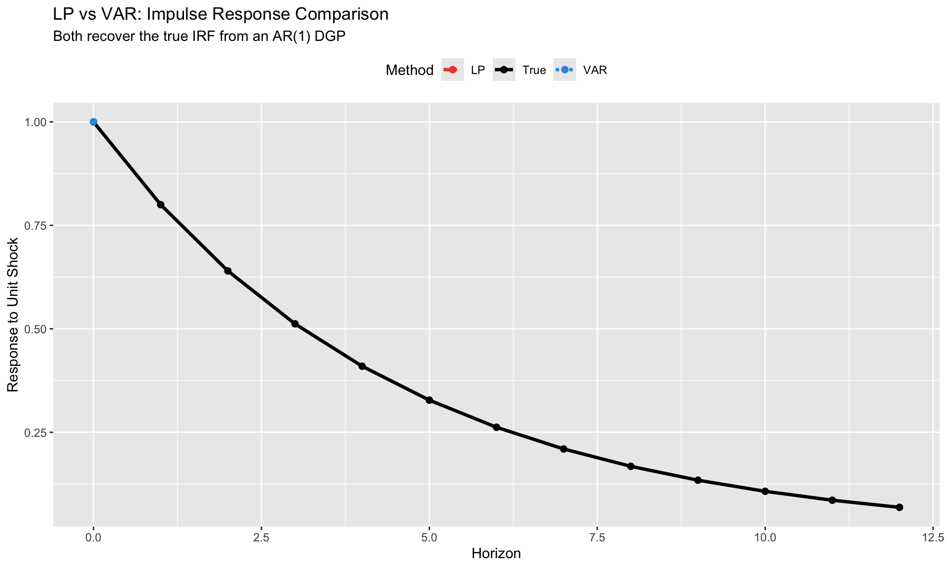
Theorem (Plagborg-Møller & Wolf, 2021): Under correct specification, LP and VAR estimate the same population impulse responses.
Both methods are consistent for: \[ \text{IRF}(h) = \frac{\partial \mathbb{E}[y_{t+h} | \mathcal{I}_t]}{\partial \text{shock}_t} \]
The difference is in finite samples and misspecification:
| Aspect | VAR | LP |
|---|---|---|
| Specification | Imposes structure | Agnostic at each horizon |
| Efficiency | More efficient if correct | Less efficient (more parameters) |
| Misspecification | Biased if wrong | Robust |
| Confidence intervals | Tighter | Wider (but honest) |
When They Diverge
LP and VAR can give different answers when:
- VAR is misspecified: Wrong lag length, omitted variables, nonlinearities
- Small samples: LP’s horizon-by-horizon estimation is noisier
- Long horizons: VAR extrapolates; LP estimates directly (sample shrinks)
Basic LP Estimation
The Specification
For a panel of countries observed over time:
\[ y_{i,t+h} - y_{i,t-1} = \alpha_i^h + \delta_t^h + \beta^h \cdot \text{shock}_{it} + \mathbf{X}_{it}'\boldsymbol{\gamma}^h + \varepsilon_{i,t+h} \]
Left-hand side: Cumulative change from \(t-1\) to \(t+h\). This gives the cumulative multiplier—how much \(y\) has changed in total by horizon \(h\).
Right-hand side: - \(\alpha_i^h\): Country fixed effects (absorb level differences) - \(\delta_t^h\): Time fixed effects (absorb common shocks) - \(\text{shock}_{it}\): The impulse of interest - \(\mathbf{X}_{it}\): Controls (lags of \(y\), other variables)
Implementation with fixest
Panel dimensions: 30 countries, 60 periods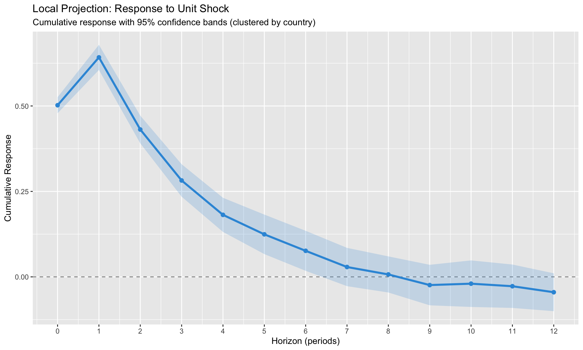
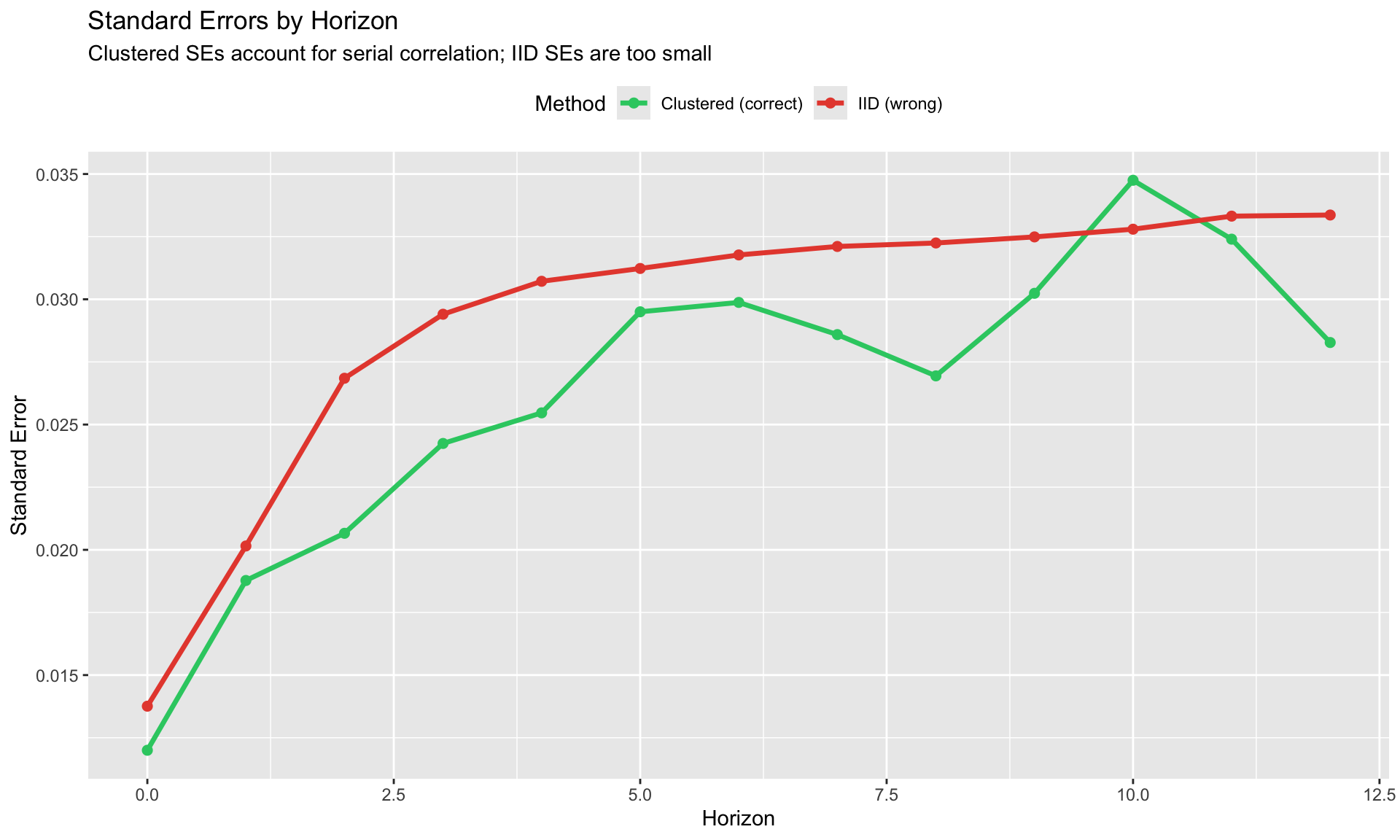
Inference: Why HAC/Clustering Matters
At horizon \(h\), the LP residual \(\varepsilon_{i,t+h}\) is correlated with \(\varepsilon_{i,t+h-1}, \ldots, \varepsilon_{i,t+1}\) by construction (overlapping observations).
This induces MA(h-1) serial correlation in errors.
Standard OLS standard errors are invalid. Must use:
| Method | When | Implementation |
|---|---|---|
| Newey-West HAC | Time series | sandwich::NeweyWest(lags = h) |
| Cluster by unit | Panel, short T | vcov = ~country |
| Driscoll-Kraay | Panel, cross-sectional dependence | vcov = "DK" in some packages |
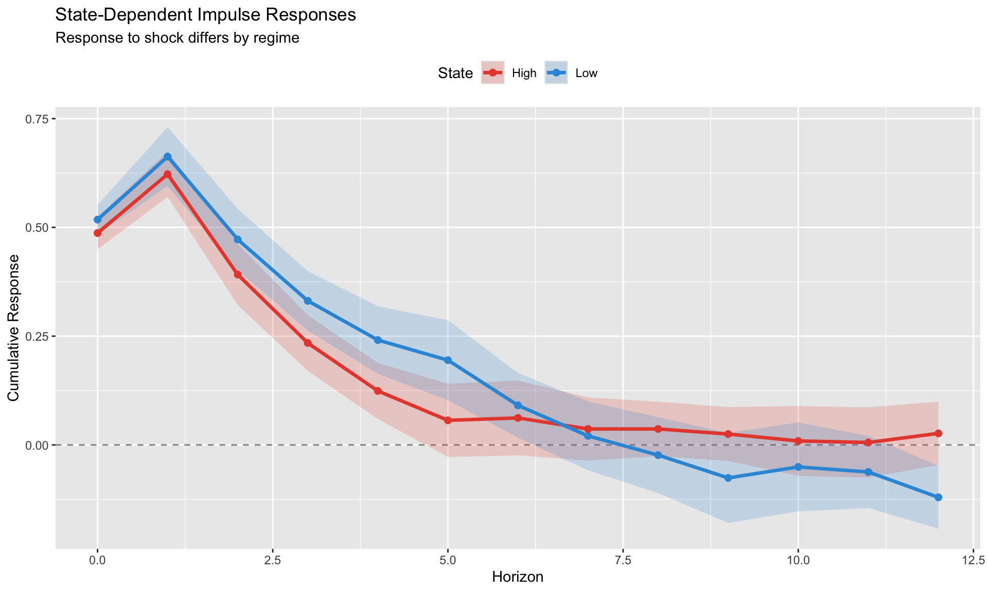
State-Dependent Local Projections
A major advantage of LP over VAR: it’s easy to allow impulse responses to vary with the state of the economy.
Binary State Switching
The simplest approach: interact the shock with a state indicator.
\[ y_{i,t+h} - y_{i,t-1} = \alpha_i^h + \beta_0^h \cdot (1 - S_{it}) \cdot \text{shock}_{it} + \beta_1^h \cdot S_{it} \cdot \text{shock}_{it} + \cdots \]
where \(S_{it} = 1\) if country \(i\) is in “state 1” at time \(t\).
Examples of state variables: - Recession vs. expansion - High vs. low debt - Financial crisis vs. normal times - High vs. low bank holdings of sovereign debt
Smooth Transition (Auerbach-Gorodnichenko)
Instead of hard switching, use a logistic function for smooth transition:
\[ F(z_t) = \frac{\exp(-\gamma z_t)}{1 + \exp(-\gamma z_t)} \]
where: - \(z_t\) is the (standardized) state variable - \(\gamma > 0\) controls transition speed - \(F(z_t) \to 1\) when \(z_t \to -\infty\) (e.g., deep recession) - \(F(z_t) \to 0\) when \(z_t \to +\infty\) (e.g., strong expansion)
The LP specification becomes:
\[ y_{t+h} = F(z_{t-1}) \cdot [\alpha_R^h + \beta_R^h \cdot \text{shock}_t] + (1 - F(z_{t-1})) \cdot [\alpha_E^h + \beta_E^h \cdot \text{shock}_t] + \cdots \]
![]()
Testing for State Dependence
To test whether responses genuinely differ across states:
\[ H_0: \beta_0^h = \beta_1^h \quad \forall h \]
Methods: 1. Joint F-test: Test equality of coefficients across horizons 2. Horizon-by-horizon t-tests: Test \(\beta_0^h - \beta_1^h = 0\) at each \(h\) 3. Cumulative difference: Test whether cumulative response differs
WarningCommon Mistake
Showing that \(\beta_0^h\) is significant and \(\beta_1^h\) is not significant does NOT prove they’re different. You must test the difference directly.
LP-DiD: Combining LP with Difference-in-Differences
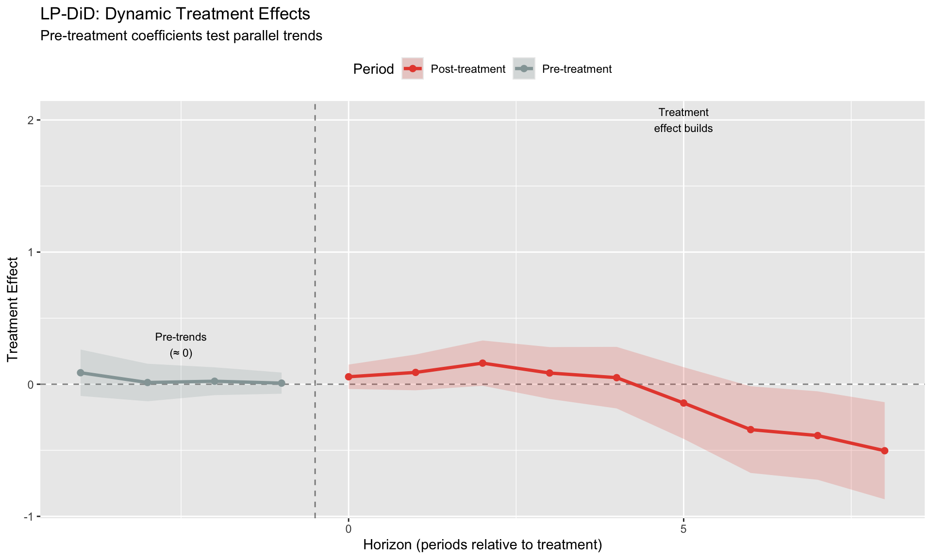
LP-DiD (Jordà, Dube, Girardi & Taylor, 2024) extends local projections to treatment effect settings with staggered adoption.
The Setting
- Some units receive treatment at different times
- We want to trace out the dynamic treatment effect at each horizon
- Standard DiD gives one number; LP-DiD gives a path
The Specification
\[ y_{i,t+h} - y_{i,t-1} = \alpha_i + \delta_t + \beta^h \cdot D_{it} + \mathbf{X}_{it}'\boldsymbol{\gamma}^h + \varepsilon_{i,t+h} \]
where: - \(D_{it} = 1\) if unit \(i\) is treated at time \(t\) - \(\alpha_i\) = unit fixed effects - \(\delta_t\) = time fixed effects - \(\beta^h\) = treatment effect at horizon \(h\)
Key features: - Estimates treatment effect at each horizon (not just one average) - Includes negative horizons to test pre-trends - Robust to heterogeneous treatment timing
LP-DiD vs. Standard Event Study
| Feature | Standard Event Study | LP-DiD |
|---|---|---|
| LHS | \(y_{it}\) | \(y_{i,t+h} - y_{i,t-1}\) |
| Interpretation | Level relative to \(t=-1\) | Cumulative change |
| Horizons | Relative time dummies | Direct projection |
| Handles dynamics | Imposes structure | Flexible |
LP-DiD is particularly useful when: - Treatment effects build gradually - You want impulse response interpretation - Dynamics are complex or nonlinear
Diagnostics and Practical Issues
Sample Erosion at Long Horizons
At horizon \(h\), you lose \(h\) observations from the end of your sample: - \(h = 0\): Full sample - \(h = 12\): Lose 12 periods (3 years of quarterly data)
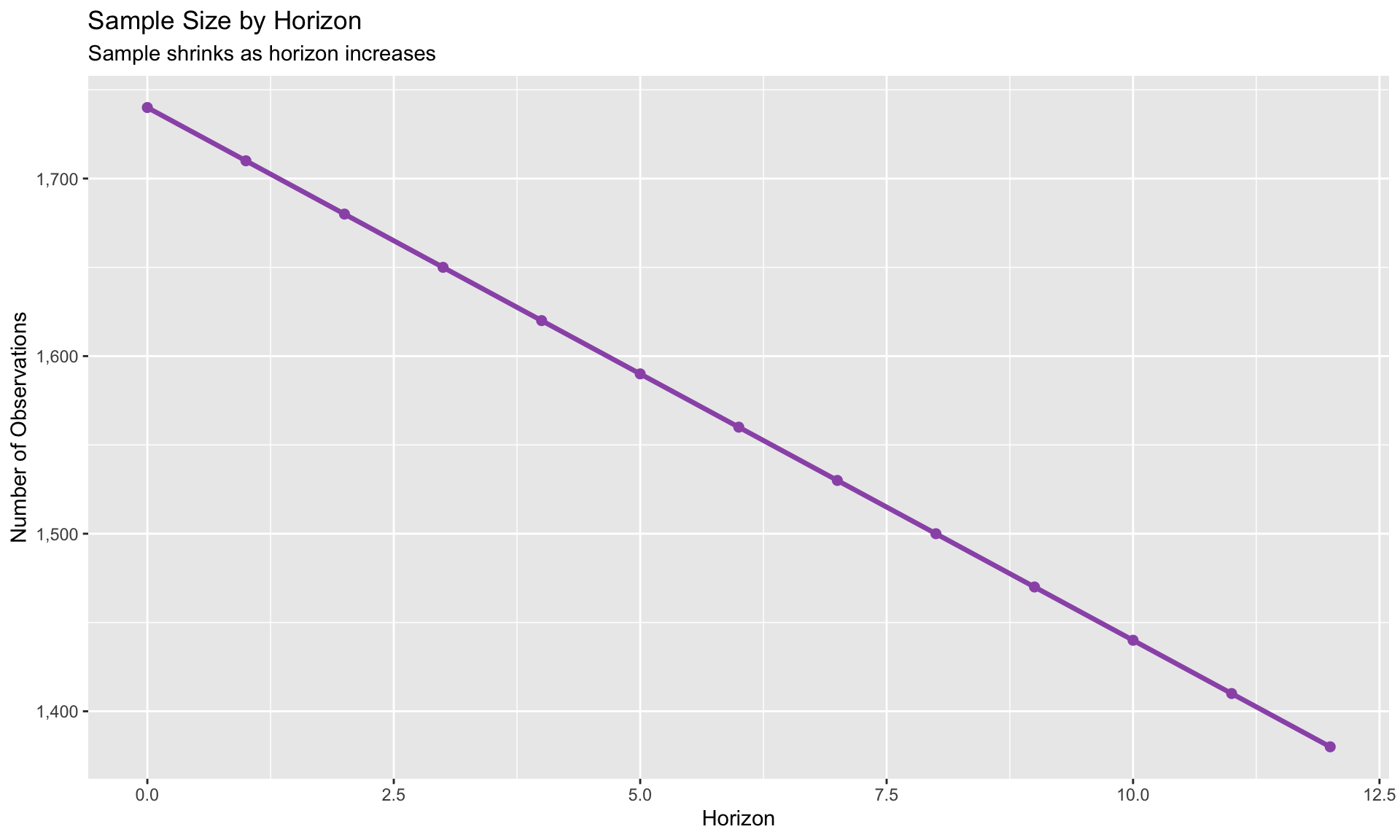
Implications: - Confidence intervals widen at longer horizons (less data + more uncertainty) - Truncate horizons when CIs become uninformative - Report effective sample size at each horizon
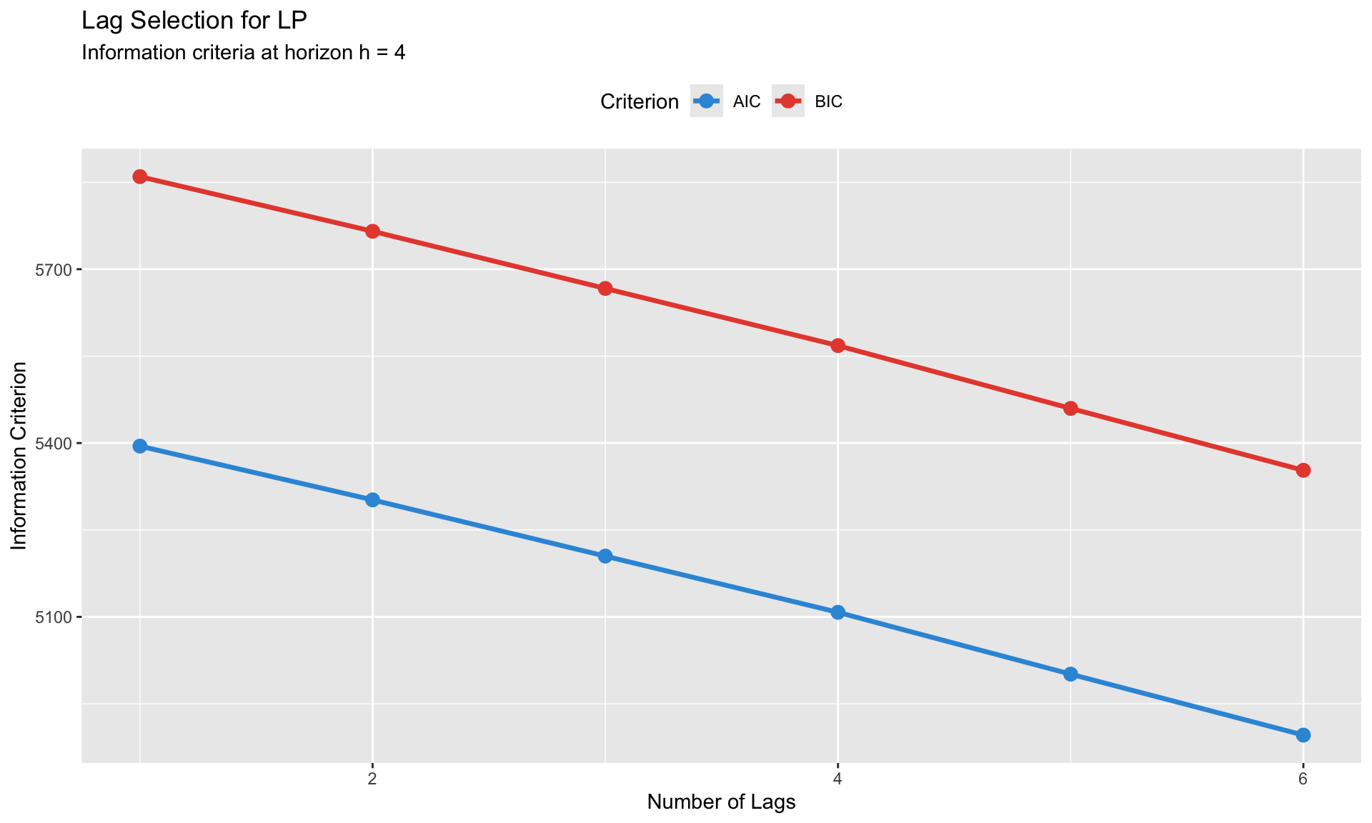
Lag Selection
Rule: Use the same lag structure across all horizons for comparability.
Methods: 1. Information criteria (AIC, BIC) on the \(h = 0\) regression 2. LM test for serial correlation in residuals 3. Rule of thumb: 2-4 lags for quarterly, 1-2 for annual
Cumulative vs. Non-Cumulative
Cumulative (recommended for levels): \[ \text{LHS} = y_{t+h} - y_{t-1} \] Interpretation: Total change from \(t-1\) to \(t+h\).
Non-cumulative: \[ \text{LHS} = y_{t+h} \] Interpretation: Level at \(t+h\) (includes pre-existing trend).
Use cumulative for: - GDP, debt/GDP, price level - Any variable where you care about the total change
Use non-cumulative for: - Growth rates, inflation (already differenced) - When you want the level effect
Comparing LP and VAR IRFs
Always compare LP and VAR when possible:
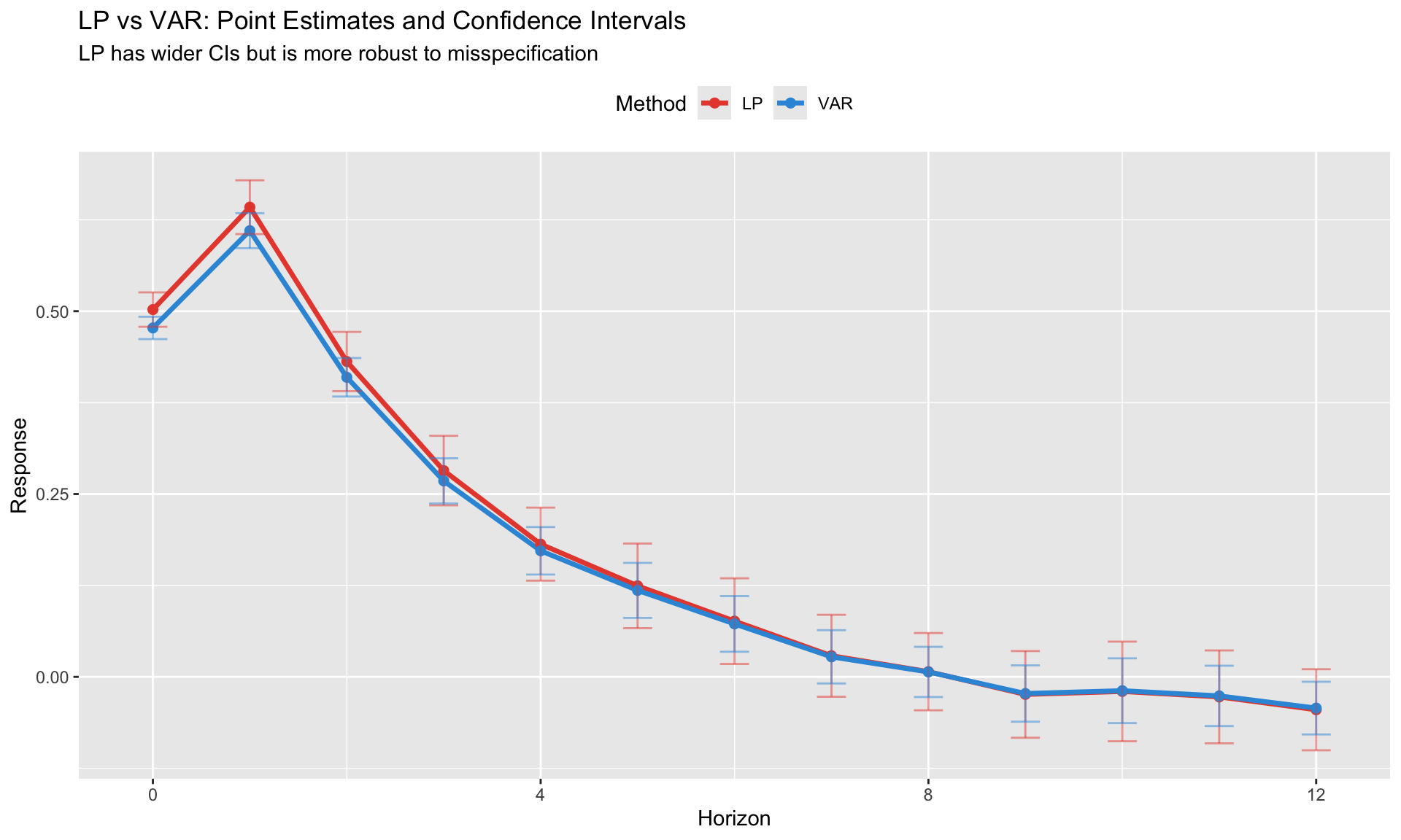
When LP and VAR disagree: - Check VAR specification (lags, variables) - LP is likely more robust to misspecification - VAR may be picking up spurious dynamics
Frequently Asked Questions
When should I use LP vs. VAR?
Use LP when: - You only need to identify ONE shock - Misspecification is a concern - You want state-dependent or nonlinear responses - You’re working with panel data
Use VAR when: - You need the full system (FEVD, historical decomposition) - Efficiency matters and you trust the specification - Short horizons with well-identified structure
How do I choose the horizon H?
- Plot IRFs and extend until they converge to zero (or steady state)
- Stop when confidence intervals become uninformative
- Rule of thumb: H = 4-5 years for quarterly macro data
- Report effective sample sizes
What controls should I include?
- Lagged dependent variable (always)
- Variables that affect both shock and outcome (confounders)
- Don’t include post-treatment controls (bad controls)
- Keep controls consistent across horizons
How do I report results?
- Plot the IRF with confidence bands
- Report the peak response and time to peak
- Table with point estimates and SEs at key horizons
- Report sample size at each horizon
- Compare with VAR if possible
Summary
Key takeaways from this module:
LP estimates IRFs directly at each horizon—no need to specify full system
LP and VAR give same population IRFs but LP is more robust to misspecification
Use HAC or clustered SEs—overlapping residuals create serial correlation
State-dependent LP is easy: interact shock with state indicator
LP-DiD extends to treatment effect settings with dynamic effects
Sample erodes at longer horizons—report effective sample sizes
Confidence intervals widen with horizon—this is a feature, not a bug