---
title: "Bayesian Vector Autoregressions"
subtitle: "Shrinkage, Minnesota Priors, and Posterior Inference"
---
```{r}
#| label: setup
#| include: false
knitr::opts_chunk$set(
echo = TRUE, warning = FALSE, message = FALSE,
fig.width = 10, fig.height = 6, fig.align = "center"
)
library(dplyr)
library(tidyr)
library(ggplot2)
library(mvtnorm)
theme_set(theme_minimal(base_size = 13))
set.seed(42)
```
# Why Bayesian VARs? {.unnumbered}
Vector Autoregressions are powerful tools for macroeconomic analysis, but they suffer from a fundamental problem: **too many parameters, too little data**.
## The Curse of Dimensionality
A VAR(p) with K variables has:
$$
\text{Parameters} = K^2 p + K = K(Kp + 1)
$$
| Variables (K) | Lags (p) | Parameters | Typical Macro Sample (T=200) |
|---------------|----------|------------|------------------------------|
| 3 | 4 | 39 | OK |
| 5 | 4 | 105 | Marginal |
| 7 | 4 | 203 | Problematic |
| 10 | 4 | 410 | Unreliable |
With quarterly data since 1960, you have ~250 observations. A 7-variable VAR(4) estimates 203 parameters—almost one parameter per observation!
```{r}
#| label: param-explosion
#| fig-cap: "The curse of dimensionality in VARs"
param_count <- expand.grid(K = 2:12, p = 1:8) %>%
mutate(params = K * (K * p + 1))
ggplot(param_count, aes(x = K, y = params, color = factor(p))) +
geom_line(linewidth = 1) +
geom_point(size = 2) +
geom_hline(yintercept = c(100, 200), linetype = "dashed", alpha = 0.5) +
annotate("text", x = 11, y = 110, label = "T = 100", hjust = 0, size = 3) +
annotate("text", x = 11, y = 210, label = "T = 200", hjust = 0, size = 3) +
scale_color_viridis_d(option = "plasma") +
labs(title = "VAR Parameters Explode with System Size",
subtitle = "Dashed lines show typical macro sample sizes",
x = "Number of Variables (K)", y = "Number of Parameters",
color = "Lags (p)")
```
## The OLS Problem
With many parameters and few observations:
- **Overfitting**: In-sample fit is excellent, out-of-sample forecasts are poor
- **Imprecision**: Huge standard errors, wide confidence intervals
- **Instability**: Small changes in data lead to large changes in estimates
## The Bayesian Solution: Shrinkage
**Key insight**: We have prior beliefs about macroeconomic dynamics. Use them!
Reasonable priors for macro VARs:
1. Variables are **persistent** (close to random walks)
2. **Own lags** matter more than other variables' lags
3. **Recent lags** matter more than distant lags
4. **Cross-variable effects** are typically small
Bayesian estimation **shrinks** estimates toward these beliefs, reducing variance at the cost of some bias. With many parameters, this variance-bias tradeoff strongly favors shrinkage.
```{r}
#| label: shrinkage-intuition
#| fig-cap: "Shrinkage reduces variance at the cost of small bias"
# Demonstrate shrinkage benefit
set.seed(123)
n_sim <- 1000
true_beta <- 0.3
n_obs <- 30
# OLS estimates (high variance)
ols_estimates <- replicate(n_sim, {
x <- rnorm(n_obs)
y <- true_beta * x + rnorm(n_obs, 0, 2)
coef(lm(y ~ x - 1))
})
# Bayesian estimates with shrinkage prior toward 0
# Prior: beta ~ N(0, 0.5^2)
prior_var <- 0.5^2
bayes_estimates <- replicate(n_sim, {
x <- rnorm(n_obs)
y <- true_beta * x + rnorm(n_obs, 0, 2)
# Posterior with known sigma = 2
sigma2 <- 4
post_var <- 1 / (1/prior_var + sum(x^2)/sigma2)
post_mean <- post_var * (sum(x*y)/sigma2)
post_mean
})
estimates_df <- data.frame(
estimate = c(ols_estimates, bayes_estimates),
method = rep(c("OLS (no shrinkage)", "Bayesian (shrinkage)"), each = n_sim)
)
ggplot(estimates_df, aes(x = estimate, fill = method)) +
geom_density(alpha = 0.5) +
geom_vline(xintercept = true_beta, linetype = "dashed", linewidth = 1) +
annotate("text", x = true_beta + 0.1, y = 1.5,
label = paste0("True β = ", true_beta), hjust = 0) +
scale_fill_manual(values = c("OLS (no shrinkage)" = "#e74c3c",
"Bayesian (shrinkage)" = "#3498db")) +
labs(title = "Shrinkage Reduces Estimation Variance",
subtitle = "Bayesian estimates cluster closer to truth despite small bias",
x = expression(hat(beta)), y = "Density",
fill = "") +
theme(legend.position = "top")
```
# The Minnesota Prior {.unnumbered}
## Litterman (1986) and Doan-Litterman-Sims (1984)
The **Minnesota prior** is the workhorse prior for macroeconomic BVARs. It encodes the belief that macro variables behave approximately like random walks.
### Prior Mean
For variables in **levels** (GDP, prices, etc.):
$$
E[A_1] = I_K, \quad E[A_j] = 0 \text{ for } j > 1
$$
Each variable's first own lag coefficient is centered at 1 (random walk), all other coefficients at 0.
For **stationary** variables (growth rates, spreads):
$$
E[A_j] = 0 \text{ for all } j
$$
### Prior Variance (The Shrinkage Structure)
The key innovation is the **structured prior variance**:
**Own lag $l$ of variable $i$**:
$$
\text{Var}(a_{ii,l}) = \left(\frac{\lambda_1}{l^d}\right)^2
$$
**Cross lag $l$ of variable $j$ on equation $i$**:
$$
\text{Var}(a_{ij,l}) = \left(\frac{\lambda_1 \cdot \lambda_2 \cdot \sigma_i}{l^d \cdot \sigma_j}\right)^2
$$
**Constant term**:
$$
\text{Var}(c_i) = (\lambda_1 \cdot \lambda_3)^2
$$
where:
- $\sigma_i$ = residual std from univariate AR(p) of variable $i$
- $\lambda_1$ = **overall tightness** (controls shrinkage strength)
- $\lambda_2$ = **cross-variable shrinkage** (typically < 1)
- $\lambda_3$ = **constant tightness** (typically large, ~100)
- $d$ = **lag decay** (typically 1 or 2)
### Hyperparameter Interpretation
| Parameter | Typical Range | Effect |
|-----------|---------------|--------|
| $\lambda_1$ | 0.1 - 0.5 | Smaller → more shrinkage toward prior |
| $\lambda_2$ | 0.3 - 0.5 | Smaller → own lags dominate cross effects |
| $\lambda_3$ | 100 | Large → loose prior on constant |
| $d$ | 1 or 2 | Larger → faster decay for distant lags |
```{r}
#| label: minnesota-variance
#| fig-cap: "Minnesota prior variance structure"
# Illustrate Minnesota prior variance structure
K <- 3
p <- 4
lambda1 <- 0.2
lambda2 <- 0.5
d <- 1
# Prior variance for different coefficient types
lags <- 1:p
own_var <- (lambda1 / lags^d)^2
cross_var <- (lambda1 * lambda2 / lags^d)^2
var_df <- data.frame(
lag = rep(lags, 2),
variance = c(own_var, cross_var),
type = rep(c("Own lag", "Cross lag"), each = p)
)
ggplot(var_df, aes(x = lag, y = sqrt(variance), color = type)) +
geom_line(linewidth = 1.2) +
geom_point(size = 3) +
scale_color_manual(values = c("Own lag" = "#3498db", "Cross lag" = "#e74c3c")) +
labs(title = "Minnesota Prior: Standard Deviation by Lag",
subtitle = expression(paste(lambda[1], " = 0.2, ", lambda[2], " = 0.5, d = 1")),
x = "Lag", y = "Prior Standard Deviation",
color = "Coefficient Type") +
theme(legend.position = "top")
```
## The Normal-Inverse-Wishart Prior
The Minnesota prior is typically implemented as a **Normal-Inverse-Wishart (NIW)** prior:
$$
\begin{aligned}
\text{vec}(B) | \Sigma &\sim N(\text{vec}(B_0), \Sigma \otimes V_0) \\
\Sigma &\sim \text{Inverse-Wishart}(S_0, \nu_0)
\end{aligned}
$$
This is **conjugate**: the posterior has the same form with updated parameters.
**Posterior**:
$$
\begin{aligned}
V_{\text{post}} &= (V_0^{-1} + X'X)^{-1} \\
B_{\text{post}} &= V_{\text{post}}(V_0^{-1} B_0 + X'Y) \\
\nu_{\text{post}} &= \nu_0 + T \\
S_{\text{post}} &= S_0 + (Y - XB_{\text{post}})'(Y - XB_{\text{post}}) + (B_{\text{post}} - B_0)'V_0^{-1}(B_{\text{post}} - B_0)
\end{aligned}
$$
# GLP: Data-Driven Hyperparameters {.unnumbered}
## Giannone, Lenza & Primiceri (2015)
How do we choose $\lambda_1, \lambda_2$? The traditional approach: researcher judgment or cross-validation.
**GLP innovation**: Choose hyperparameters by **maximizing the marginal likelihood**:
$$
p(Y | \lambda) = \int p(Y | B, \Sigma) \cdot p(B, \Sigma | \lambda) \, dB \, d\Sigma
$$
For the NIW prior, this integral has a **closed-form solution**!
### The Algorithm
1. Define a grid over $\lambda = (\lambda_1, \lambda_2, \ldots)$
2. For each $\lambda$, compute $p(Y | \lambda)$ analytically
3. Choose $\lambda^* = \arg\max_\lambda p(Y | \lambda)$
4. Estimate BVAR with optimal hyperparameters
### Why This Matters
- **Data-driven**: No arbitrary hyperparameter choices
- **Automatic**: Adapts to different datasets
- **Forecast accuracy**: GLP BVARs consistently outperform OLS VARs
```{r}
#| label: glp-illustration
#| fig-cap: "GLP marginal likelihood optimization"
# Illustrate marginal likelihood as function of lambda
# (Simulated for illustration)
lambda_grid <- seq(0.01, 1, length.out = 50)
# Simulated marginal likelihood (realistic shape)
set.seed(42)
ml_values <- -50 - 20*(lambda_grid - 0.25)^2 + rnorm(50, 0, 2)
ml_df <- data.frame(lambda = lambda_grid, log_ml = ml_values)
optimal_lambda <- lambda_grid[which.max(ml_values)]
ggplot(ml_df, aes(x = lambda, y = log_ml)) +
geom_line(linewidth = 1, color = "#3498db") +
geom_vline(xintercept = optimal_lambda, linetype = "dashed", color = "#e74c3c") +
annotate("point", x = optimal_lambda, y = max(ml_values),
size = 4, color = "#e74c3c") +
annotate("text", x = optimal_lambda + 0.05, y = max(ml_values) - 5,
label = paste0("λ* = ", round(optimal_lambda, 2)), hjust = 0,
color = "#e74c3c") +
labs(title = "GLP: Marginal Likelihood Optimization",
subtitle = "Optimal shrinkage is data-determined",
x = expression(lambda[1] ~ "(Overall Tightness)"),
y = "Log Marginal Likelihood")
```
## Additional Priors: Sum-of-Coefficients and No-Cointegration
GLP (2015) also optimizes over additional priors that improve forecasting:
### Sum-of-Coefficients (Doan-Litterman-Sims)
Belief: If all variables equal their sample means, the forecast should also be the mean.
Implemented by adding dummy observations. Controlled by hyperparameter $\mu$.
### No-Cointegration (Sims-Zha)
Belief: Variables have unit roots but are not cointegrated.
Also implemented via dummy observations. Controlled by hyperparameter $\delta$.
**GLP jointly optimizes** $(\lambda_1, \lambda_2, \mu, \delta)$ via marginal likelihood.
# Gibbs Sampling for BVAR {.unnumbered}
While the NIW prior allows analytical posteriors, we often use **Gibbs sampling** to:
- Easily compute posterior quantities (IRFs, FEVDs)
- Extend to non-conjugate priors
- Handle structural identification
## The Gibbs Sampler
**Block 1**: Draw $B | \Sigma, Y$
$$
\text{vec}(B) | \Sigma, Y \sim N(\text{vec}(B_{\text{post}}), \Sigma \otimes V_{\text{post}})
$$
**Block 2**: Draw $\Sigma | B, Y$
$$
\Sigma | B, Y \sim \text{Inverse-Wishart}(S_{\text{post}}, \nu_{\text{post}})
$$
Iterate for $G$ draws, discarding the first $B_{\text{burn}}$ as burn-in.
```{r}
#| label: gibbs-bvar
#| fig-cap: "Gibbs sampler trace plots for BVAR coefficient"
# Simplified BVAR Gibbs sampler demonstration
# Generate synthetic VAR(1) data
T_obs <- 100
K <- 2
# True parameters
A_true <- matrix(c(0.8, 0.1, 0.05, 0.7), K, K)
Sigma_true <- matrix(c(1, 0.3, 0.3, 1), K, K)
# Generate data
Y <- matrix(0, T_obs, K)
Y[1, ] <- rnorm(K)
for (t in 2:T_obs) {
Y[t, ] <- Y[t-1, ] %*% t(A_true) + rmvnorm(1, sigma = Sigma_true)
}
# Build matrices
y <- Y[2:T_obs, ]
X <- cbind(1, Y[1:(T_obs-1), ])
T_eff <- nrow(y)
M <- ncol(X)
# Minnesota-style prior
B0 <- matrix(0, M, K)
B0[2:3, ] <- diag(K) * 0.9 # Prior: close to random walk
# Prior precision (diagonal, tight) - must be (M*K) x (M*K) for vec(B)
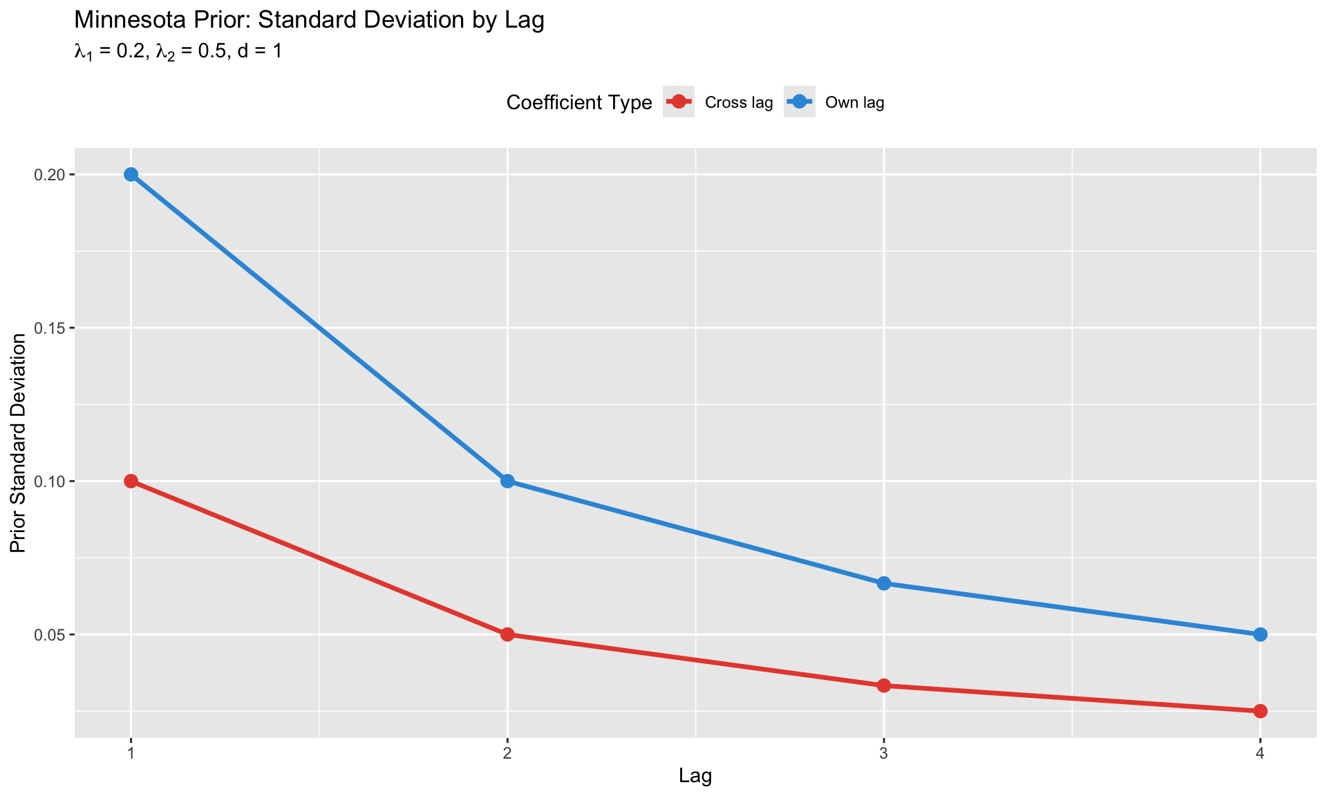
lambda1 <- 0.2
# Build prior variance for each coefficient in vec(B)
# Structure: [const_eq1, y1_eq1, y2_eq1, const_eq2, y1_eq2, y2_eq2]
v0_diag <- numeric(M * K)
for (eq in 1:K) {
idx_const <- (eq - 1) * M + 1
v0_diag[idx_const] <- 100 # Loose prior on constant
for (var in 1:K) {
idx_var <- (eq - 1) * M + 1 + var
v0_diag[idx_var] <- lambda1^2 # Tight prior on AR coefficients
}
}
V0_inv <- diag(1 / v0_diag)
# Prior for Sigma
nu0 <- K + 2
S0 <- diag(K)
# Gibbs sampler
n_draw <- 2000
n_burn <- 500
B_draws <- array(0, dim = c(M, K, n_draw))
Sigma_draws <- array(0, dim = c(K, K, n_draw))
# Initialize
B_curr <- solve(crossprod(X)) %*% crossprod(X, y)
Sigma_curr <- crossprod(y - X %*% B_curr) / T_eff
for (g in 1:(n_draw + n_burn)) {
# Draw B | Sigma using vectorized form
# vec(B) | Sigma ~ N(b_post, V_post) where V_post = (V0_inv + Sigma^{-1} ⊗ X'X)^{-1}
Sigma_inv <- solve(Sigma_curr)
V_post_inv <- V0_inv + kronecker(Sigma_inv, crossprod(X))
V_post <- solve(V_post_inv)
b_post <- V_post %*% (V0_inv %*% as.vector(B0) +
kronecker(Sigma_inv, t(X)) %*% as.vector(y))
B_curr <- matrix(rmvnorm(1, b_post, V_post), M, K)
# Draw Sigma | B
U <- y - X %*% B_curr
S_post <- S0 + crossprod(U)
Sigma_curr <- solve(rWishart(1, nu0 + T_eff, solve(S_post))[,,1])
# Store
if (g > n_burn) {
B_draws[,,g - n_burn] <- B_curr
Sigma_draws[,,g - n_burn] <- Sigma_curr
}
}
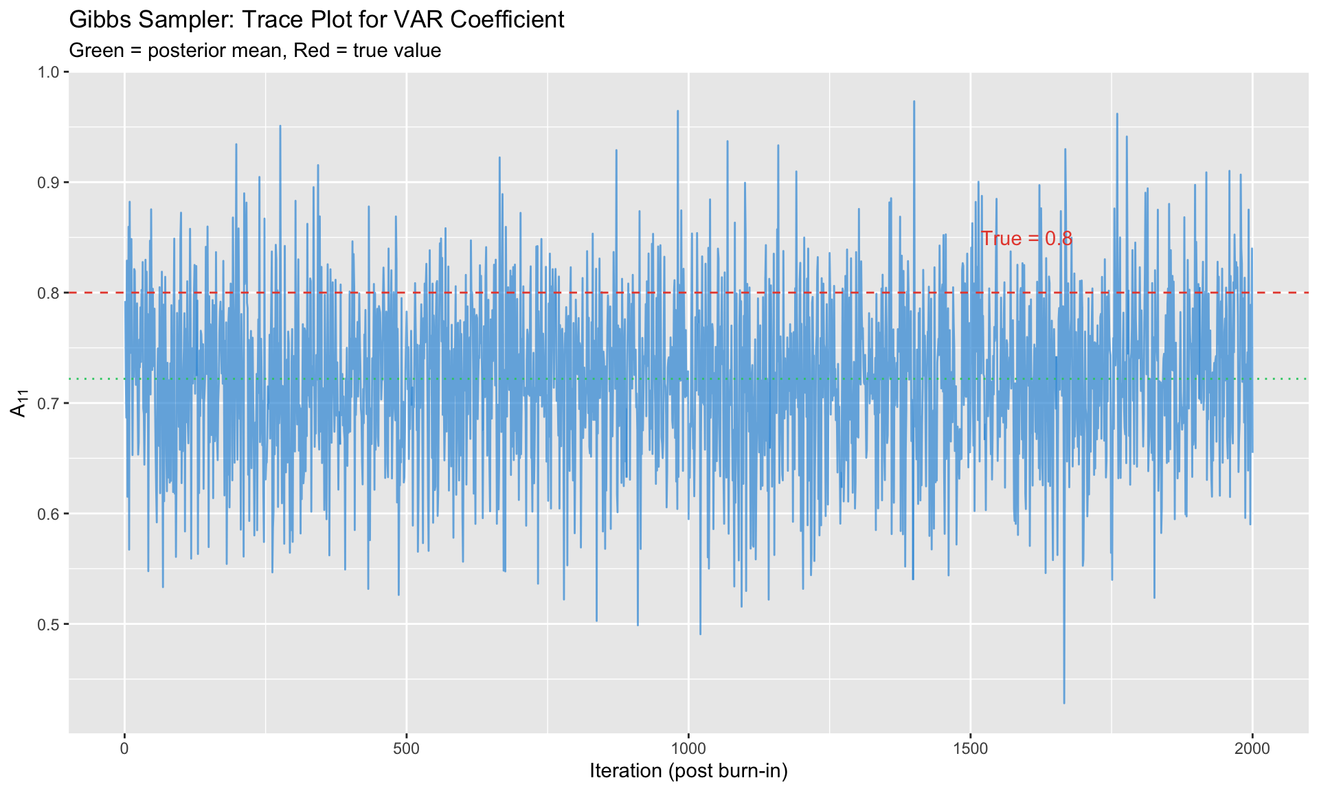
# Trace plot for A[1,1]
trace_df <- data.frame(
iteration = 1:n_draw,
value = B_draws[2, 1, ] # A[1,1] coefficient
)
ggplot(trace_df, aes(x = iteration, y = value)) +
geom_line(alpha = 0.7, color = "#3498db") +
geom_hline(yintercept = A_true[1,1], linetype = "dashed", color = "#e74c3c") +
geom_hline(yintercept = mean(trace_df$value), linetype = "dotted", color = "#2ecc71") +
annotate("text", x = n_draw * 0.8, y = A_true[1,1] + 0.05,
label = paste0("True = ", A_true[1,1]), color = "#e74c3c") +
labs(title = "Gibbs Sampler: Trace Plot for VAR Coefficient",
subtitle = "Green = posterior mean, Red = true value",
x = "Iteration (post burn-in)", y = expression(A[11]))
```
# Structural Identification in BVAR {.unnumbered}
Bayesian VARs estimate **reduced-form** parameters $(B, \Sigma)$. For structural analysis, we need to identify structural shocks.
## Cholesky Identification
The simplest approach: impose a recursive structure.
$$
\Sigma = PP', \quad P = \text{chol}(\Sigma, \text{lower})
$$
For each posterior draw $\Sigma^{(g)}$, compute $P^{(g)} = \text{chol}(\Sigma^{(g)})$.
The ordering matters: variable ordered first is not affected contemporaneously by others.
## Sign Restrictions in BVAR
Bayesian framework naturally handles set-identification:
1. For each posterior draw $(B^{(g)}, \Sigma^{(g)})$:
a. Compute $P^{(g)} = \text{chol}(\Sigma^{(g)})$
b. Draw orthogonal rotation $Q$ uniformly
c. Candidate impact: $\tilde{P}^{(g)} = P^{(g)} Q$
d. Check sign restrictions on IRFs
e. If satisfied: keep. Otherwise: redraw $Q$
2. Report distribution across accepted draws
```{r}
#| label: sign-restrictions
# Sign restriction: monetary tightening
# - Raises interest rate (positive)
# - Lowers output (negative)
# - Lowers inflation (negative)
restrictions <- data.frame(
Variable = c("Interest Rate", "Output", "Inflation"),
Sign = c("+", "-", "-"),
Interpretation = c("Policy instrument", "Demand falls", "Prices fall")
)
knitr::kable(restrictions,
caption = "Example Sign Restrictions for Monetary Policy Shock")
```
# IRFs and FEVDs from Posterior {.unnumbered}
## Computing Posterior IRFs
For each posterior draw $(B^{(g)}, \Sigma^{(g)})$:
1. Extract coefficient matrices $A_1^{(g)}, \ldots, A_p^{(g)}$ from $B^{(g)}$
2. Compute structural impact $P^{(g)}$ (Cholesky or sign-restricted)
3. Compute IRF at each horizon using MA representation:
$$
\Phi_h = \sum_{j=1}^{\min(h,p)} \Phi_{h-j} A_j, \quad \Phi_0 = I
$$
4. Structural IRF: $\text{IRF}_h = \Phi_h P$
Report **posterior median** and **credible bands** (68%, 95%).
```{r}
#| label: posterior-irfs
#| fig-cap: "Impulse responses with posterior credible bands"
# Compute IRFs from Gibbs draws
H <- 20 # horizons
K <- 2
n_draws_use <- 500 # use subset for speed
IRF_draws <- array(0, dim = c(K, K, H+1, n_draws_use))
for (g in 1:n_draws_use) {
# Extract A matrix (coefficients on lagged Y)
A1 <- t(B_draws[2:3, , g])
# Cholesky impact
P <- t(chol(Sigma_draws[,,g]))
# Compute IRFs
Phi <- diag(K)
IRF_draws[,,1,g] <- P
for (h in 1:H) {
Phi <- Phi %*% A1
IRF_draws[,,h+1,g] <- Phi %*% P
}
}
# Extract IRF of variable 1 to shock 1
irf_11 <- IRF_draws[1, 1, , ]
# Posterior summaries
irf_median <- apply(irf_11, 1, median)
irf_lower <- apply(irf_11, 1, quantile, 0.16)
irf_upper <- apply(irf_11, 1, quantile, 0.84)
irf_lower95 <- apply(irf_11, 1, quantile, 0.025)
irf_upper95 <- apply(irf_11, 1, quantile, 0.975)
irf_df <- data.frame(
horizon = 0:H,
median = irf_median,
lower68 = irf_lower,
upper68 = irf_upper,
lower95 = irf_lower95,
upper95 = irf_upper95
)
ggplot(irf_df, aes(x = horizon)) +
geom_ribbon(aes(ymin = lower95, ymax = upper95), fill = "#3498db", alpha = 0.2) +
geom_ribbon(aes(ymin = lower68, ymax = upper68), fill = "#3498db", alpha = 0.4) +
geom_line(aes(y = median), linewidth = 1.2, color = "#2c3e50") +
geom_hline(yintercept = 0, linetype = "dashed") +
labs(title = "Bayesian VAR: Impulse Response Function",
subtitle = "Posterior median with 68% and 95% credible bands",
x = "Horizon", y = "Response of Y1 to Shock 1")
```
## Forecast Error Variance Decomposition
FEVD at horizon $h$:
$$
\text{FEVD}_{i,j}(h) = \frac{\sum_{s=0}^{h} (\text{IRF}_{i,j,s})^2}{\sum_{s=0}^{h} \sum_{k=1}^{K} (\text{IRF}_{i,k,s})^2}
$$
Compute for each posterior draw, report median and bands.
# Implementation in R {.unnumbered}
## Using the `BVAR` Package
The `BVAR` package implements Minnesota priors with GLP-style optimization.
```r
library(BVAR)
# Prepare data (T × K matrix)
data_mat <- as.matrix(macro_data[, c("gdp_growth", "inflation", "interest_rate")])
# Minnesota prior with GLP optimization
mn_prior <- bv_minnesota(
lambda = bv_lambda(mode = 0.2, sd = 0.4, min = 0.0001, max = 5),
alpha = bv_alpha(mode = 2), # lag decay
var = 1e07 # constant variance
)
# Estimate BVAR
bvar_model <- bvar(
data = data_mat,
lags = 4,
n_draw = 20000,
n_burn = 5000,
priors = mn_prior,
mh = bv_mh(scale_hess = 0.01, adjust_acc = TRUE)
)
# Diagnostics
summary(bvar_model)
plot(bvar_model) # trace plots
# IRFs (Cholesky identification)
irf_results <- irf(bvar_model, horizon = 20, identification = TRUE)
plot(irf_results)
# FEVD
fevd_results <- fevd(bvar_model, horizon = 20)
plot(fevd_results)
# Forecasting
forecasts <- predict(bvar_model, horizon = 8)
plot(forecasts)
```
## Using the `bvartools` Package
More flexible, allows custom prior specification.
```r
library(bvartools)
# Generate VAR data matrices
bvar_data <- gen_var(data_ts, p = 4, deterministic = "const")
y <- t(bvar_data$data$Y)
x <- t(bvar_data$data$Z)
# Set up Minnesota prior manually
K <- ncol(data_mat)
M <- K * 4 + 1
# Prior mean: random walk on first lag
a_mu_prior <- matrix(0, M, K)
a_mu_prior[2:(K+1), ] <- diag(K)
# Prior precision (Minnesota structure)
a_v_i_prior <- diag(1, M * K) * 0.01
# Prior for Sigma
u_sigma_df_prior <- K + 2
u_sigma_scale_prior <- diag(1, K)
# Estimate
bvar_est <- bvar(
y = y, x = x,
A = list(mu = a_mu_prior, V_i = a_v_i_prior),
Sigma = list(df = u_sigma_df_prior, scale = u_sigma_scale_prior),
iterations = 20000, burnin = 5000
)
# IRFs
bvar_irf <- irf(bvar_est,
impulse = "interest_rate",
response = "inflation",
n.ahead = 20,
type = "feir", # forecast error IRF
ci = 0.95)
plot(bvar_irf)
```
## Manual Implementation
For full control and understanding:
```r
bvar_gibbs <- function(Y, p, n_draw = 10000, n_burn = 2000,
lambda1 = 0.2, lambda2 = 0.5, lambda3 = 100) {
T_full <- nrow(Y)
K <- ncol(Y)
M <- K * p + 1
# Build data matrices
y <- Y[(p + 1):T_full, ]
T_eff <- nrow(y)
X <- cbind(1)
for (j in 1:p) {
X <- cbind(X, Y[(p + 1 - j):(T_full - j), ])
}
# Minnesota prior mean
B0 <- matrix(0, M, K)
B0[2:(K + 1), ] <- diag(K) # first lag = identity
# Scaling from AR residuals
sigma_i <- numeric(K)
for (i in 1:K) {
ar_fit <- ar(Y[, i], order.max = p, method = "ols")
sigma_i[i] <- sqrt(ar_fit$var.pred)
}
# Prior variance (Minnesota structure)
V0_diag <- numeric(M * K)
for (eq in 1:K) {
idx <- (eq - 1) * M + 1
V0_diag[idx] <- (lambda1 * lambda3)^2 # constant
for (lag in 1:p) {
for (var in 1:K) {
idx <- (eq - 1) * M + 1 + (lag - 1) * K + var
if (var == eq) {
V0_diag[idx] <- (lambda1 / lag)^2
} else {
V0_diag[idx] <- (lambda1 * lambda2 * sigma_i[eq] / (lag * sigma_i[var]))^2
}
}
}
}
V0_inv <- diag(1 / V0_diag)
# Inverse Wishart prior
v0 <- K + 2
S0 <- diag(sigma_i^2)
# Storage and initialization
B_draws <- array(0, dim = c(M, K, n_draw))
Sigma_draws <- array(0, dim = c(K, K, n_draw))
B_curr <- solve(crossprod(X)) %*% crossprod(X, y)
Sigma_curr <- crossprod(y - X %*% B_curr) / T_eff
# Gibbs sampler
for (g in 1:(n_draw + n_burn)) {
# Block 1: B | Sigma
Sigma_inv <- solve(Sigma_curr)
V_post_inv <- V0_inv + kronecker(Sigma_inv, crossprod(X))
V_post <- solve(V_post_inv)
b_post <- V_post %*% (V0_inv %*% as.vector(B0) +
kronecker(Sigma_inv, t(X)) %*% as.vector(y))
B_curr <- matrix(mvtnorm::rmvnorm(1, b_post, V_post), M, K)
# Block 2: Sigma | B
U <- y - X %*% B_curr
S_post <- S0 + crossprod(U)
v_post <- v0 + T_eff
Sigma_curr <- solve(rWishart(1, v_post, solve(S_post))[,,1])
if (g > n_burn) {
B_draws[,,g - n_burn] <- B_curr
Sigma_draws[,,g - n_burn] <- Sigma_curr
}
}
list(B = B_draws, Sigma = Sigma_draws, K = K, p = p)
}
```
# Implementation in Python {.unnumbered}
For those who prefer Python, here are equivalent implementations.
## Using NumPy/SciPy (Manual)
```python
import numpy as np
from scipy import stats
from scipy.linalg import cholesky, solve
def bvar_gibbs(Y, p, n_draw=10000, n_burn=2000,
lambda1=0.2, lambda2=0.5, lambda3=100):
"""
Bayesian VAR with Minnesota prior via Gibbs sampling.
Parameters
----------
Y : ndarray (T, K)
Data matrix
p : int
Lag order
n_draw : int
Number of posterior draws
n_burn : int
Burn-in period
lambda1, lambda2, lambda3 : float
Minnesota prior hyperparameters
Returns
-------
dict with posterior draws of B and Sigma
"""
T_full, K = Y.shape
M = K * p + 1
# Build data matrices
y = Y[p:]
T_eff = len(y)
X = np.ones((T_eff, 1))
for j in range(1, p + 1):
X = np.hstack([X, Y[p-j:T_full-j]])
# Minnesota prior mean (random walk on first lag)
B0 = np.zeros((M, K))
B0[1:K+1, :] = np.eye(K)
# AR residual scaling
sigma_i = np.zeros(K)
for i in range(K):
ar_resid = Y[p:, i] - Y[p-1:-1, i] * 0.9 # approximate
sigma_i[i] = np.std(ar_resid)
# Prior variance (Minnesota structure)
V0_diag = np.zeros(M * K)
for eq in range(K):
idx = eq * M
V0_diag[idx] = (lambda1 * lambda3)**2
for lag in range(1, p + 1):
for var in range(K):
idx = eq * M + 1 + (lag - 1) * K + var
if var == eq:
V0_diag[idx] = (lambda1 / lag)**2
else:
V0_diag[idx] = (lambda1 * lambda2 * sigma_i[eq] /
(lag * sigma_i[var]))**2
V0_inv = np.diag(1 / V0_diag)
# Inverse Wishart prior
v0 = K + 2
S0 = np.diag(sigma_i**2)
# Initialize
B_curr = np.linalg.lstsq(X, y, rcond=None)[0]
U = y - X @ B_curr
Sigma_curr = U.T @ U / T_eff
# Storage
B_draws = np.zeros((M, K, n_draw))
Sigma_draws = np.zeros((K, K, n_draw))
for g in range(n_draw + n_burn):
# Block 1: Draw B | Sigma
Sigma_inv = np.linalg.inv(Sigma_curr)
V_post_inv = V0_inv + np.kron(Sigma_inv, X.T @ X)
V_post = np.linalg.inv(V_post_inv)
b0_vec = B0.flatten('F')
xy_vec = (X.T @ y @ Sigma_inv).flatten('F')
b_post = V_post @ (V0_inv @ b0_vec + xy_vec)
B_curr = np.random.multivariate_normal(b_post, V_post).reshape((M, K), order='F')
# Block 2: Draw Sigma | B
U = y - X @ B_curr
S_post = S0 + U.T @ U
v_post = v0 + T_eff
# Inverse Wishart draw
Sigma_curr = stats.invwishart.rvs(df=v_post, scale=S_post)
if g >= n_burn:
B_draws[:, :, g - n_burn] = B_curr
Sigma_draws[:, :, g - n_burn] = Sigma_curr
return {'B': B_draws, 'Sigma': Sigma_draws, 'K': K, 'p': p}
def compute_irfs(bvar_result, shock_idx, H=20):
"""
Compute IRFs from BVAR posterior draws.
"""
B_draws = bvar_result['B']
Sigma_draws = bvar_result['Sigma']
K = bvar_result['K']
p = bvar_result['p']
n_draw = B_draws.shape[2]
IRF_draws = np.zeros((K, H + 1, n_draw))
for g in range(n_draw):
# Extract A matrices
A = [B_draws[1 + j*K:1 + (j+1)*K, :, g].T for j in range(p)]
# Cholesky impact
P = cholesky(Sigma_draws[:, :, g], lower=True)
# Compute IRFs
Phi = np.eye(K)
IRF_draws[:, 0, g] = P[:, shock_idx]
for h in range(1, H + 1):
Phi = Phi @ A[0] if p >= 1 else np.zeros((K, K))
IRF_draws[:, h, g] = Phi @ P[:, shock_idx]
return {
'median': np.median(IRF_draws, axis=2),
'lower': np.percentile(IRF_draws, 16, axis=2),
'upper': np.percentile(IRF_draws, 84, axis=2)
}
```
## Using PyMC (Probabilistic Programming)
```python
import pymc as pm
import numpy as np
import arviz as az
def bvar_pymc(Y, p, n_draw=2000, n_tune=1000):
"""
Bayesian VAR using PyMC.
"""
T_full, K = Y.shape
# Build data matrices
y = Y[p:]
T_eff = len(y)
X = np.ones((T_eff, 1))
for j in range(1, p + 1):
X = np.hstack([X, Y[p-j:T_full-j]])
M = X.shape[1]
with pm.Model() as bvar_model:
# Priors
# Coefficients: Normal with Minnesota-style shrinkage
B = pm.Normal('B', mu=0, sigma=0.5, shape=(M, K))
# Covariance: LKJ prior on correlation + half-normal on scales
chol, corr, stds = pm.LKJCholeskyCov(
'chol', n=K, eta=2, sd_dist=pm.HalfNormal.dist(sigma=1)
)
Sigma = pm.Deterministic('Sigma', chol @ chol.T)
# Likelihood
mu = pm.math.dot(X, B)
y_obs = pm.MvNormal('y', mu=mu, chol=chol, observed=y)
# Sample
trace = pm.sample(n_draw, tune=n_tune, cores=2,
return_inferencedata=True)
return trace
# Usage:
# trace = bvar_pymc(Y, p=4)
# az.plot_trace(trace, var_names=['B'])
# az.summary(trace, var_names=['B', 'Sigma'])
```
# Summary {.unnumbered}
Key takeaways:
1. **Why Bayesian VAR**: Shrinkage prevents overfitting when parameters outnumber observations
2. **Minnesota Prior**: Encodes beliefs that macro variables are persistent, own lags dominate, recent lags matter more
3. **GLP Optimization**: Data-driven hyperparameter selection via marginal likelihood maximization
4. **Gibbs Sampling**: Iteratively draw $B|\Sigma$ and $\Sigma|B$ from conditional posteriors
5. **Structural Identification**: Cholesky (recursive) or sign restrictions, applied to each posterior draw
6. **Reporting**: Present posterior median IRFs with 68% and 95% credible bands
7. **Software**:
- R: `BVAR` (GLP optimization), `bvartools` (flexible), `bvarsv` (TVP-VAR)
- Python: Manual with NumPy/SciPy, or PyMC for probabilistic programming
---
## Key References
**Foundational**:
- Litterman (1986). "Forecasting with Bayesian VARs." *JBES*
- Doan, Litterman & Sims (1984). "Forecasting and Conditional Projection."
- Sims & Zha (1998). "Bayesian Methods for Dynamic Multivariate Models." *IER*
**Modern Methods**:
- Giannone, Lenza & Primiceri (2015). "Prior Selection for VARs." *REStat*
- Banbura, Giannone & Reichlin (2010). "Large Bayesian VARs." *JAE*
- Carriero, Clark & Marcellino (2019). "Large BVARs with Stochastic Volatility." *JoE*
**Textbooks**:
- Koop (2003). *Bayesian Econometrics*
- Blake & Mumtaz (2012). *Applied Bayesian Econometrics for Central Bankers*
**R Packages**:
- `BVAR`: Kuschnig & Vashold — Minnesota prior with GLP
- `bvartools`: Mohr — Flexible BVAR toolkit
- `bvarsv`: Krueger — TVP-VAR with stochastic volatility
---
*Next: [Module 9: Bayesian Panel Methods](09_bayesian_panel.qmd)*