Regularization for Macro
LASSO, Ridge, Elastic Net, and High-Dimensional Methods
The High-Dimensional Challenge
Modern macroeconomics faces a dimensionality problem:
- Many potential predictors (hundreds of macro indicators)
- Short time series (T = 50-200 quarters)
- Traditional methods overfit: \(K > T\) makes OLS infeasible
NoteThe Core Trade-off
Bias-variance trade-off: More flexible models fit training data better but may generalize poorly. Regularization adds bias to reduce variance.
When Regularization Matters
| Setting | Problem | Solution |
|---|---|---|
| Large VARs | K variables → K²p parameters | Minnesota prior (shrinkage) |
| Forecasting | Many predictors, short samples | LASSO/Ridge selection |
| Factor models | High-dimensional data | PCA, factor extraction |
| Causal inference | Many potential confounders | Double LASSO |
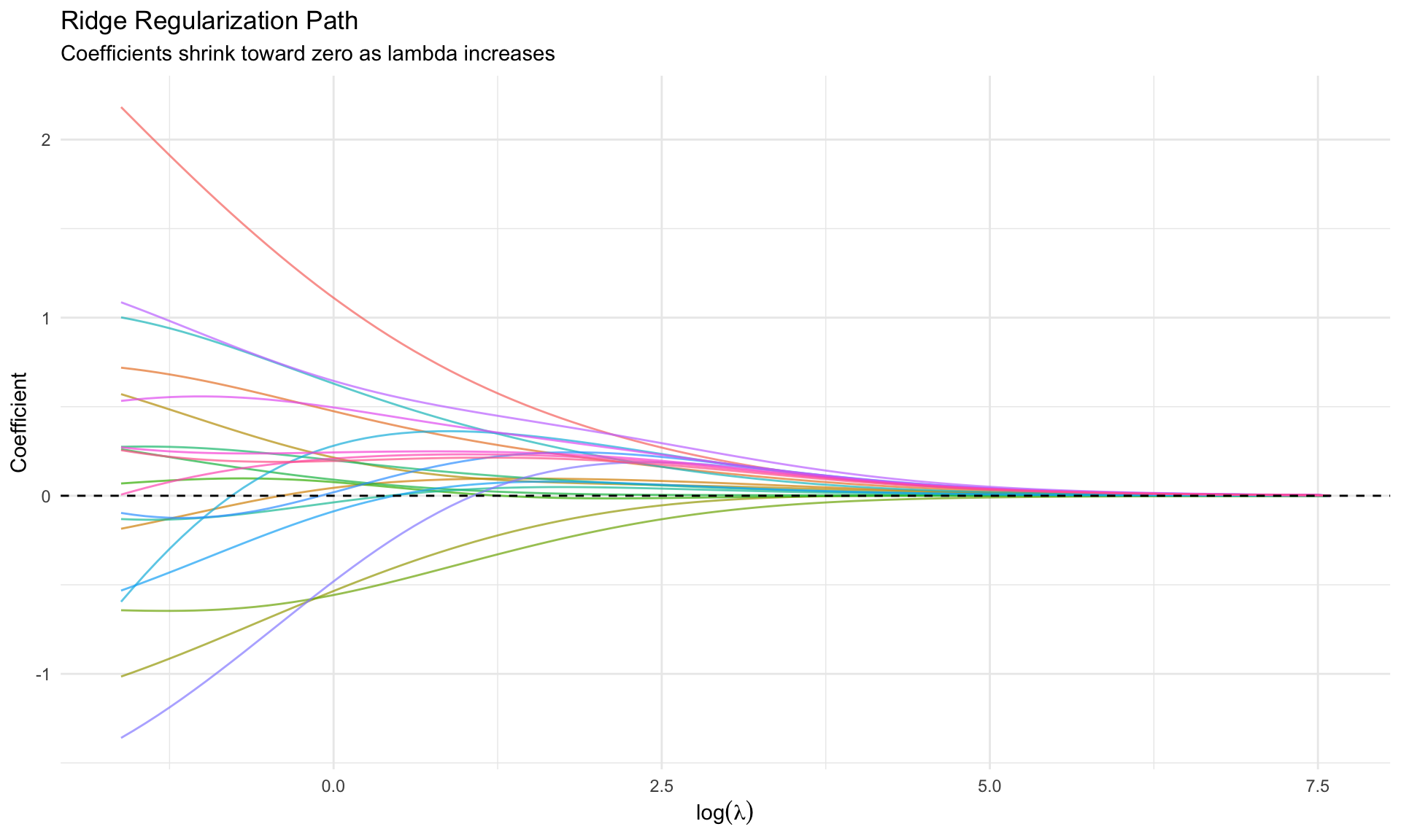
Ridge Regression
The Idea
Add an \(\ell_2\) penalty to prevent coefficients from exploding:
\[ \hat{\beta}^{\text{ridge}} = \arg\min_\beta \left\{ \sum_{i=1}^n (y_i - x_i'\beta)^2 + \lambda \sum_{j=1}^p \beta_j^2 \right\} \]
Equivalently: \[ \hat{\beta}^{\text{ridge}} = (X'X + \lambda I)^{-1} X'y \]
Key Properties
| Property | Implication |
|---|---|
| Shrinks toward zero | All coefficients are shrunk |
| Never exactly zero | Does NOT do variable selection |
| Continuous | Stable, smooth as function of \(\lambda\) |
| Handles multicollinearity | \((X'X + \lambda I)\) always invertible |
Connection to Bayesian Priors
Ridge regression is equivalent to Bayesian regression with: \[ \beta_j \sim N(0, \tau^2), \quad \tau^2 = \frac{\sigma^2}{\lambda} \]
This is exactly the Minnesota prior intuition: shrink toward zero with tightness \(\lambda\).
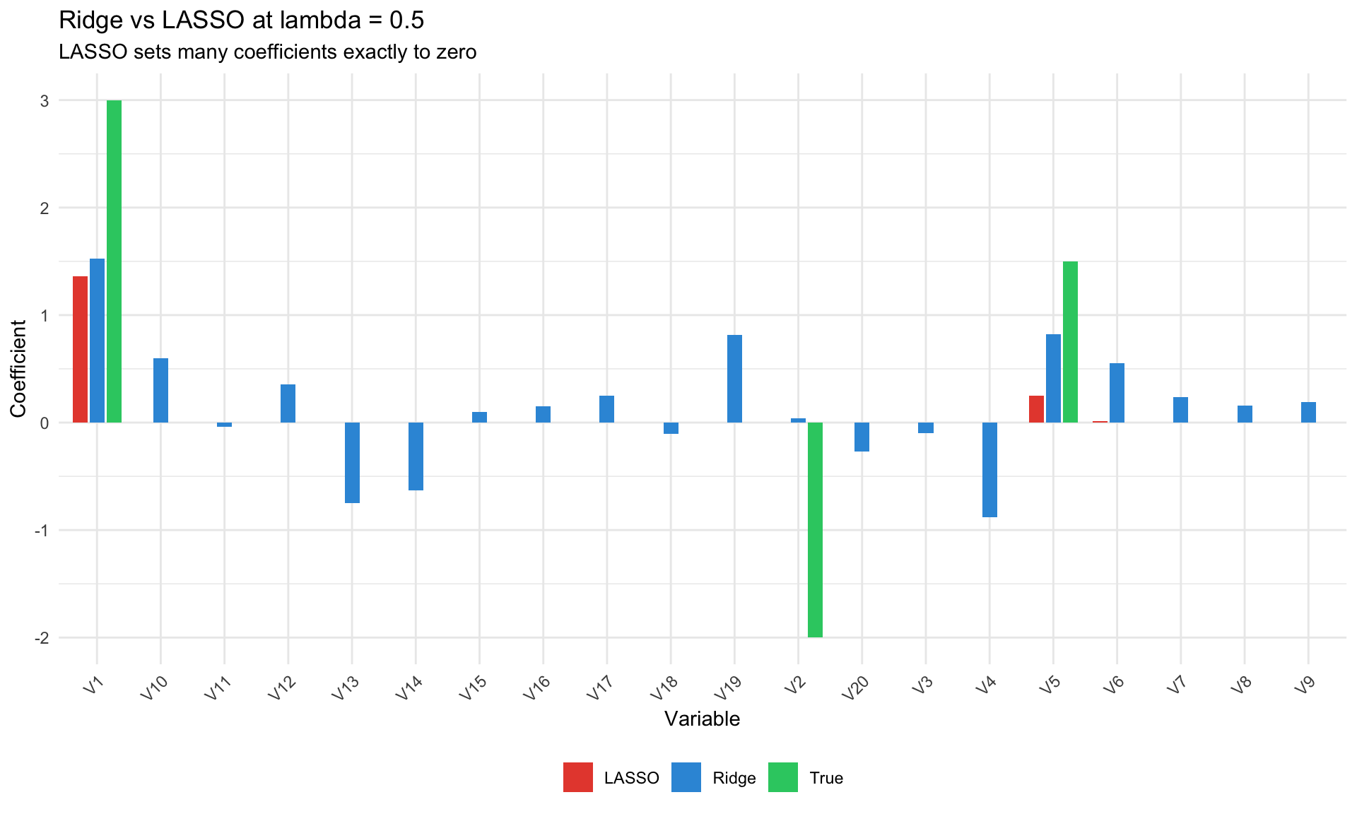
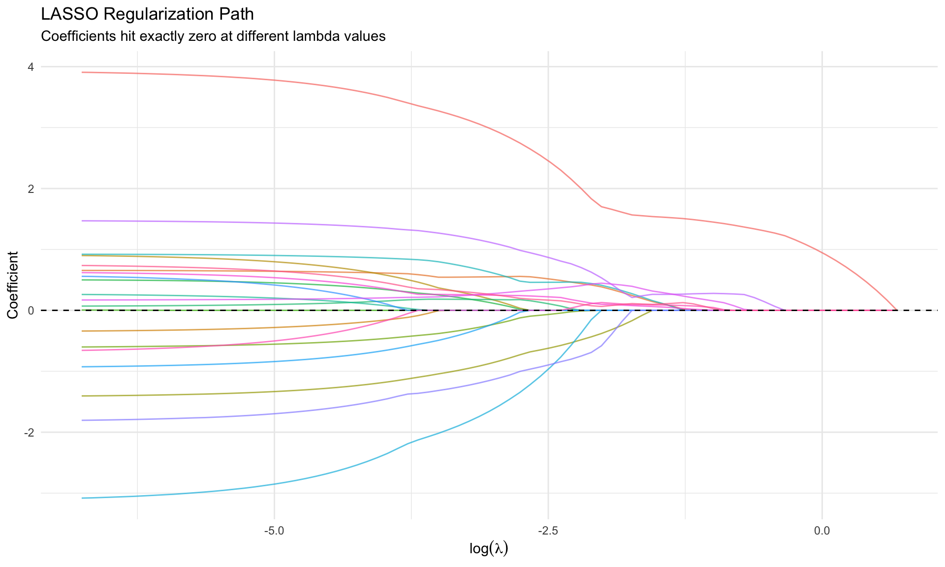
LASSO
The Idea
Replace \(\ell_2\) penalty with \(\ell_1\) (absolute value):
\[ \hat{\beta}^{\text{LASSO}} = \arg\min_\beta \left\{ \sum_{i=1}^n (y_i - x_i'\beta)^2 + \lambda \sum_{j=1}^p |\beta_j| \right\} \]
Key Properties
| Property | Implication |
|---|---|
| Shrinks to exactly zero | Automatic variable selection |
| Sparse solutions | Most coefficients are zero |
| Non-smooth | Path has kinks (not differentiable) |
| Selects one from correlated group | Arbitrary among correlated predictors |
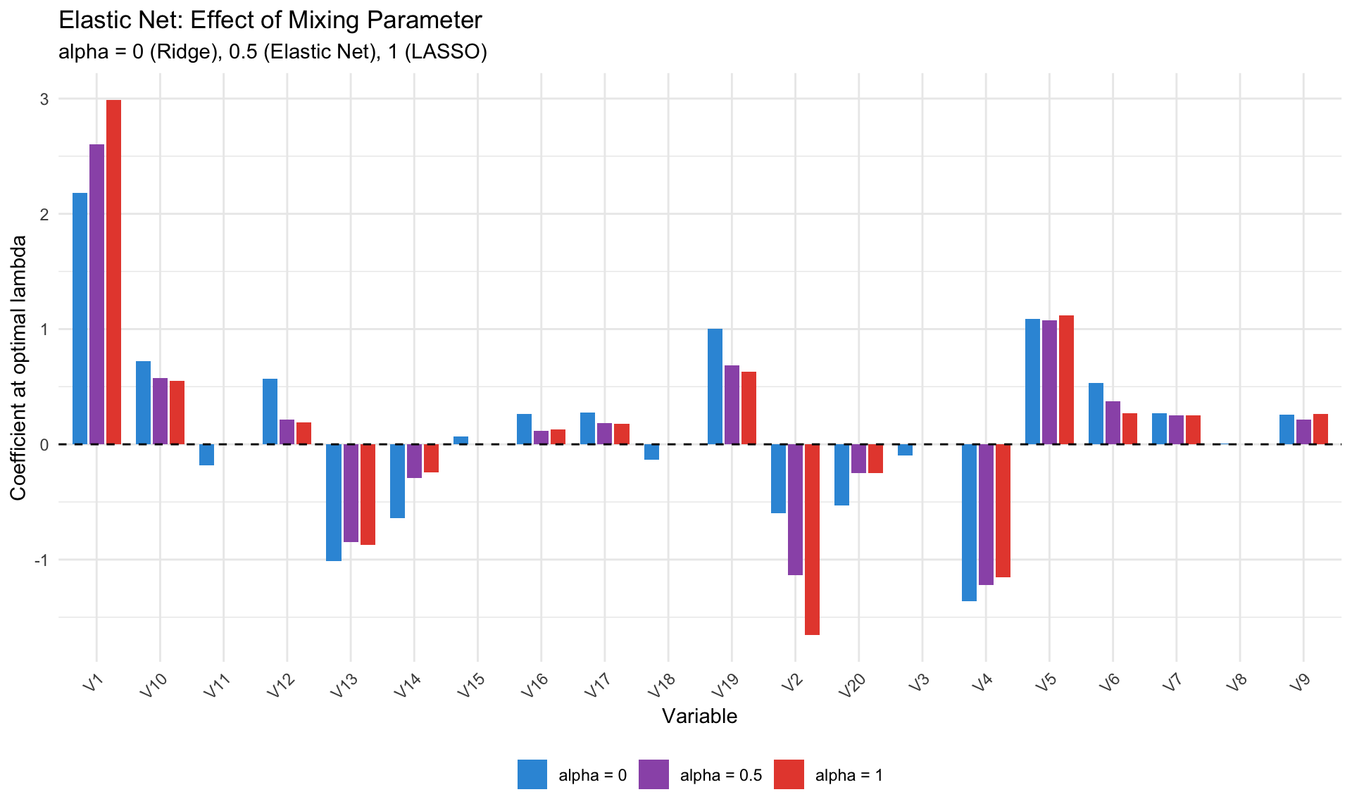
Elastic Net
Combining Ridge and LASSO
\[ \hat{\beta}^{\text{EN}} = \arg\min_\beta \left\{ \sum_{i=1}^n (y_i - x_i'\beta)^2 + \lambda \left[ \alpha \sum_j |\beta_j| + (1-\alpha) \sum_j \beta_j^2 \right] \right\} \]
| \(\alpha\) | Method |
|---|---|
| 0 | Ridge |
| 1 | LASSO |
| 0.5 | Elastic Net (balanced) |
When to Use Elastic Net
- Correlated predictors: LASSO arbitrarily selects one; Elastic Net keeps groups together
- \(p > n\): LASSO selects at most \(n\) variables; Elastic Net can select more
- Default in practice: Often use \(\alpha = 0.5\) as a robust choice
Choosing Lambda: Cross-Validation
K-Fold Cross-Validation
- Split data into K folds
- For each \(\lambda\):
- Train on K-1 folds, predict on held-out fold
- Repeat K times
- Average prediction error
- Choose \(\lambda\) that minimizes CV error
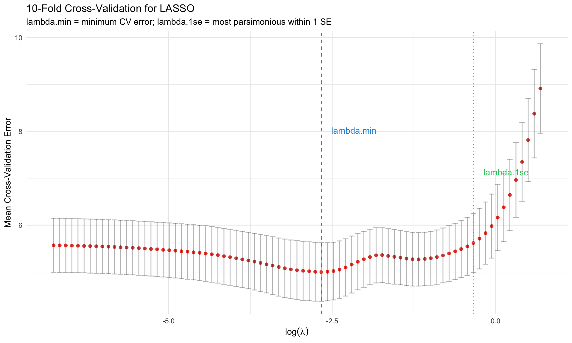
lambda.min vs lambda.1se
| Choice | Description | When to Use |
|---|---|---|
lambda.min |
Minimizes CV error | Maximum predictive power |
lambda.1se |
Largest \(\lambda\) within 1 SE of min | More parsimonious, often preferred |
Double/Debiased LASSO
The Problem with Naive LASSO for Inference
LASSO gives biased estimates and invalid standard errors because:
- Regularization bias: Shrinkage toward zero
- Model selection uncertainty: Which variables are “truly” zero?
- No valid confidence intervals in the classical sense
The Solution: Double Selection
For causal effect of \(D\) on \(Y\) with high-dimensional controls \(X\):
Step 1: LASSO of \(Y\) on \(X\) → select controls \(\hat{S}_Y\)
Step 2: LASSO of \(D\) on \(X\) → select controls \(\hat{S}_D\)
Step 3: OLS of \(Y\) on \(D\) and \(\hat{S}_Y \cup \hat{S}_D\)
This is the Belloni, Chernozhukov, Hansen (2014) approach.
Naive OLS (biased): 2.581 Double LASSO: 1.976 True effect: 2 Selected variables: 4 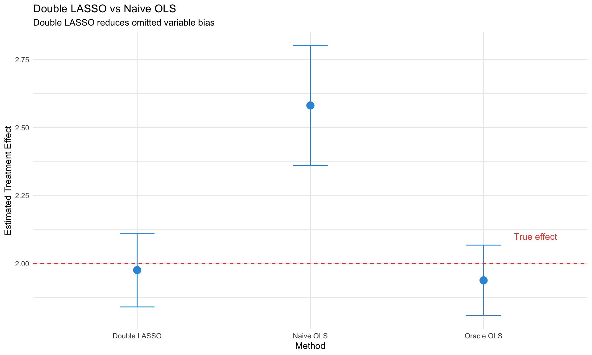
The hdm Package in R
library(hdm)

# Double selection
ds_result <- rlassoEffect(x = X, y = Y, d = D, method = "double selection")
summary(ds_result)

# Partialling out
po_result <- rlassoEffect(x = X, y = Y, d = D, method = "partialling out")
summary(po_result)
Applications in Macro
Large Bayesian VARs (Banbura, Giannone, Reichlin 2010)
Problem: K-variable VAR(p) has \(K^2 p\) parameters.
Solution: Tighter Minnesota prior as dimension grows
\[ \lambda_1^{\text{large}} = \lambda_1^{\text{small}} \times \frac{K_{\text{small}}}{K_{\text{large}}} \]
This is implicit Ridge regularization.
Factor-Augmented VAR (FAVAR)
Extract factors from large dataset, include in VAR:
\[ \begin{pmatrix} F_t \\ Y_t \end{pmatrix} = A \begin{pmatrix} F_{t-1} \\ Y_{t-1} \end{pmatrix} + u_t \]
where \(F_t\) are principal components of hundreds of macro series.
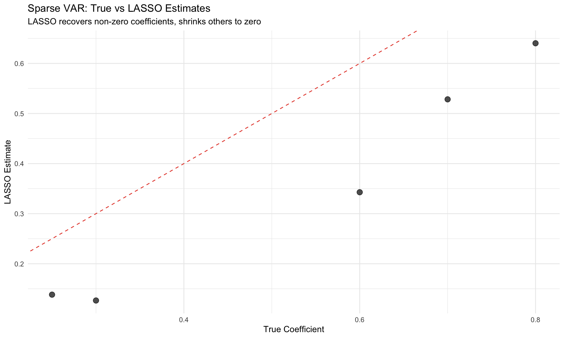
Sparse Granger Causality
Use LASSO to identify which variables Granger-cause others in high-dimensional settings.
Practical Implementation
The glmnet Workflow
library(glmnet)

# Standardize predictors (glmnet does this internally)
X <- scale(X)

# Ridge (alpha = 0)
ridge_fit <- glmnet(X, y, alpha = 0)
cv_ridge <- cv.glmnet(X, y, alpha = 0)
coef(cv_ridge, s = "lambda.min")

# LASSO (alpha = 1)
lasso_fit <- glmnet(X, y, alpha = 1)
cv_lasso <- cv.glmnet(X, y, alpha = 1)
coef(cv_lasso, s = "lambda.1se")

# Elastic Net (alpha = 0.5)
en_fit <- glmnet(X, y, alpha = 0.5)
cv_en <- cv.glmnet(X, y, alpha = 0.5)

# Predictions
predict(cv_lasso, newx = X_new, s = "lambda.min")
Choosing Alpha
Use nested cross-validation:
# Grid search over alpha
alpha_grid <- seq(0, 1, 0.1)
cv_errors <- sapply(alpha_grid, function(a) {
cv_fit <- cv.glmnet(X, y, alpha = a)
min(cv_fit$cvm)
})
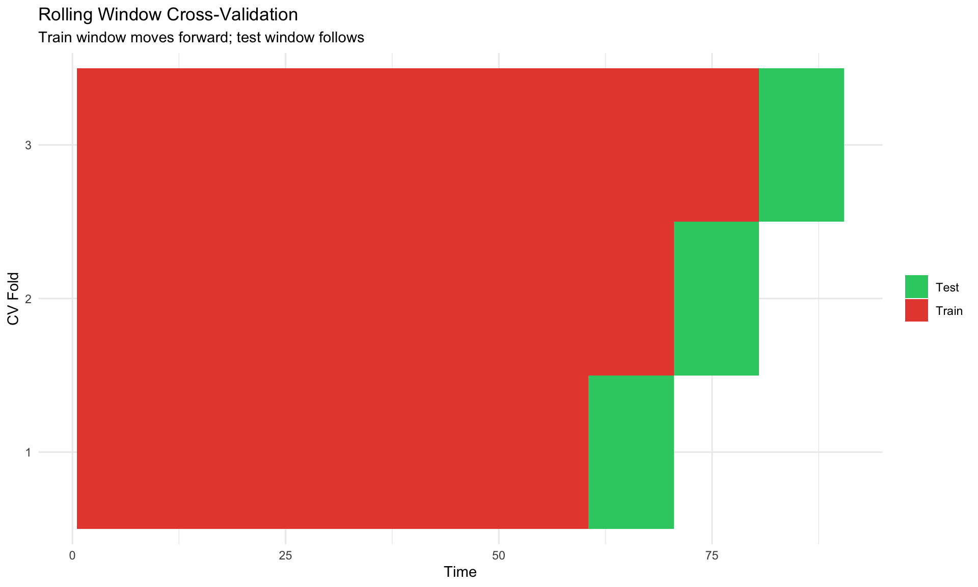
best_alpha <- alpha_grid[which.min(cv_errors)]Time Series Considerations
Standard CV is problematic for time series (breaks temporal structure).
Solutions:
- Rolling window CV: Train on \(t=1,\ldots,s\), test on \(s+1,\ldots,s+h\)
- Expanding window CV: Train on \(t=1,\ldots,s\), test on \(s+1\), then expand
- Block bootstrap: Resample blocks to preserve autocorrelation
Common Pitfalls
WarningWatch Out For
- Post-selection inference: Don’t report OLS standard errors after LASSO selection
- Standardization: Always standardize predictors for fair penalization
- Time series CV: Don’t use random splits for time series
- Interpretation: LASSO coefficients are shrunken—not the “true” effects
- Correlated predictors: LASSO picks arbitrarily; consider Elastic Net
- Oracle property: LASSO is consistent under stringent conditions (irrepresentable condition)
Summary
| Method | Penalty | Selection | When to Use |
|---|---|---|---|
| Ridge | \(\ell_2\) | No | Multicollinearity, all predictors matter |
| LASSO | \(\ell_1\) | Yes | Sparse truth, variable selection |
| Elastic Net | Both | Yes | Correlated predictors, \(p > n\) |
| Double LASSO | \(\ell_1\) | Yes | Causal inference with many controls |
TipFor Macro Applications
- Forecasting: LASSO/Ridge with rolling CV
- Large VARs: Minnesota prior (implicit Ridge)
- Causal inference: Double LASSO for high-dimensional controls
- Model selection: Elastic Net as robust default
Key References
Regularization Methods
- Tibshirani (1996) “Regression Shrinkage and Selection via the Lasso” JRSS-B
- Zou & Hastie (2005) “Regularization and Variable Selection via the Elastic Net” JRSS-B
- Hastie, Tibshirani & Wainwright (2015) Statistical Learning with Sparsity — Comprehensive textbook
High-Dimensional Inference
- Belloni, Chernozhukov & Hansen (2014) “Inference on Treatment Effects after Selection” RES — Double LASSO
- Chernozhukov et al. (2018) “Double/Debiased Machine Learning” Econometrics Journal
- Athey & Imbens (2019) “Machine Learning Methods That Economists Should Know About” Annual Review
Macro Applications
- Banbura, Giannone & Reichlin (2010) “Large Bayesian VARs” JAE
- Stock & Watson (2012) “Generalized Shrinkage Methods for Forecasting” JAE
- Giannone, Lenza & Primiceri (2021) “Economic Predictions with Big Data” JAE
Software
- glmnet: Friedman, Hastie & Tibshirani — R package for penalized regression
- hdm: Chernozhukov et al. — High-dimensional metrics in R